

I was asked by a reader if I could illustrate the application of the Kalman Filter technique described in my previous post with an example. Let’s take the ETF pair AGG IEF, using daily data from Jan 2006 to Feb 2015 to estimate the model. As you can see from the chart in Fig. 1, the pair have been highly correlated over the last several years.
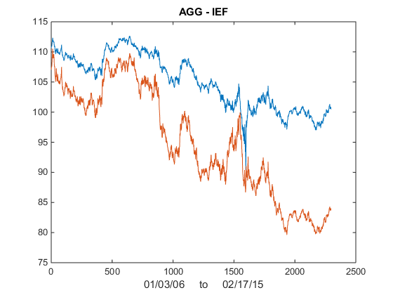 Fig 1. AGG and IEF Daily Prices 2006-2015
We now estimate the beta-relationship between the ETF pair with the Kalman Filter, using the Matlab code given below, and plot the estimated vs actual prices of the first ETF, AGG in Fig 2. There are one or two outliers that you might want to take a look at, but mostly the fit looks very good. 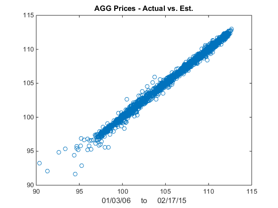
Fig 2 – Actual vs Fitted Prices of AGG
Now lets take a look at Kalman Filter estimates of beta. As you can see in Fig 3, it wanders around a lot! Very difficult to handle using some kind of static beta estimate. 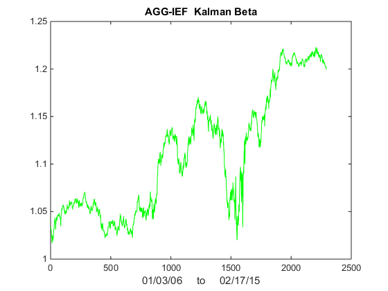
Fig 3 – Kalman Filter Beta Estimates
Finally, we compute the raw and standardized alphas, being the differences between the observed and fitted prices , i.e. Alpha(t) = AGG(t) – b(t)* IEF(t) and kfAlpha(t) = (Alpha(t) – mean(Alpha(t)) / std(Alpha(t) I have plotted the kfAlpha estimates over the last year in Fig 4. 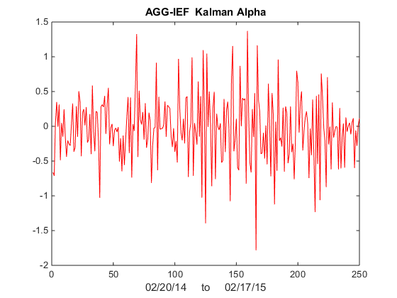
Fig 4 – Standardized Alpha Estimates
The last step is to decide how to trade this relationship. You might, for example, trade the portfolio in proportion to the standardized deviation (i.e. the size of kfAlpha(t)). Alternatively, you might set a threshold level, say +/- 1 Sd, and trade the portfolio when kfAlpha(t) exceeds this the threshold. In the Matlab code below I use the particle swarm method to maximize the likelihood. I have found this to be more reliable than other methods.
%
function [QR, distAlpha, kfBeta, Pt,Yhat, Alpha, kfAlpha, Lik] = estimateKalmanBeta(QR0,varargin)
%
%%%%%%%%%%%%%%%%%%%%%%%%%%%%%%%%%%%%%%%%%%%%%%%%%%%%%%%%%%%%%%%%%%%%%%%%%%%'
%%%%%%%%%%%%%%%%%%%%%%%%%%%%%%%%%%%%%%%%%%%%%%%%%%%%%%%%%%%%%%%%%%%%%%%%%%%'
%
%               ETF STATISTICAL ARBITARGE STRATEGY
%                           VERSION 2.2.2
%                   JONATHAN KINLAY JAN 15, 2015
%
%%%%%%%%%%%%%%%%%%%%%%%%%%%%%%%%%%%%%%%%%%%%%%%%%%%%%%%%%%%%%%%%%%%%%%%%%%%'
%%%%%%%%%%%%%%%%%%%%%%%%%%%%%%%%%%%%%%%%%%%%%%%%%%%%%%%%%%%%%%%%%%%%%%%%%%%'
% USAGE:
%
% [QR, distAlpha, kfBeta,Yhat, Alpha, kfAlpha, Lik]] =
%            estimateKalmanBeta_ver_2_1_1(Y, X, QR0)
%
% SYSTEM DYNAMICS:
%
% The system evolves according to the following difference equations,
% where quantities are further defined below:
%
% b(t) = b(t-1) + w     Beta, the unobserved state variable
%                       follows a random walk
% Y(t) = b(t)X(t) + v   The observed processes of stock prices
%                        Y(t) and X(t)
% where w ~ N(0,Q) meaning w is gaussian noise with variance Q
%       v ~ N(0,R) meaning v is gaussian noise with variance R
%
% The signal noise ratio Q/R is critical, generally around 1E-6/1E-7
%
%
% =========================================================================
%INPUTS:
%
% QR0(1x2)                  - initial estimates of Q and R
%
% Prices (nobs x 2)          - Matrix of prices
%  OR
% [Y(nobs,1) X(nobs,2)]       - two, single column vectors of prices
%
% =========================================================================
%OUTPUTS:
%
% QR(1)                     - updated estimate of variance Q
% QR(2)                     - updated estimate of variance R
%
% distaAlpha(1)             - estimated mean of Alpha
% distAlpha (2)             - estimated std of Alpha
%
% kfBeta(nobs,1)            - vector of beta(t) estimates
%
% Pt                        - see eqn below
%
% Yhat(nobs x 1)            - vector of estimated Y(t) prices
%
% Alpha(nobs x 1)           - vector of Alpha(t)=Y(t) - Yhat(t)
%
% kfAlpha(nobs x 1)         - vector of standardized alpha(t)
%
% Lik (scalar)              - estimated likelihood function value

if nargin < 3
    Prices=cell2mat(varargin(1));
    Y=Prices(:,1);
    X=Prices(:,2);
else
    Y=cell2mat(varargin(1));
    X=cell2mat(varargin(2));
end
cleanPrices = [Y,X];
cleanPrices = cleanPrices(~any(isnan(cleanPrices),2),:);
nobs = length(Y);
kfBeta=ones(nobs,1);
Yhat=NaN(nobs,1);

if ~isnan(Y(1)) && ~isnan(X(1))
    kfBeta(1)=Y(1)/X(1);
end
Yhat(1) = Y(1);
Pt=0;
%
%%%%%%%%%%%%%%%%%  GA OPTIMIZATION %%%%%%%%%%%%%%
%
%kfBetaLik = @(QR)kfBetaLikelihood(Y, X, QR);
%options = gaoptimset('Generations', 60, 'TolFun', 1E-10);
%[QR, Lik] = ga(kfBetaLik, 2,[],[],[],[],[0 0], [0.1 0.1],[],options);
%%%%%%%%%%%%%%%%%%%%%%%%%%%%%%%%%%%%%%%%%%%%%%%%%%%
%
%%%%%%%%%%%%%%%%%%%%%%%%%%%%%%%%%%%%%%%%%%%%%%%%%%%
%%%%%%%%%%  PARTICLE SWARM OPTIMIZATION %%%%%%%%%%%
%
kfBetaLik = @(QR)kfBetaLikelihood(cleanPrices(:,1), cleanPrices(:,2), QR);
options = optimoptions('particleswarm','SwarmSize',100,'HybridFcn',@fmincon,'TolFun', 1E-10, 'Display', 'off');
[QR, Lik] = particleswarm(kfBetaLik, 2,[0 0], [1 1],options);
%%%%%%%%%%%%%%%%%%%%%%%%%%%%%%%%%%%%%%%%%%%%%%%%%%%
%
%
Q=QR(1);
R=QR(2);
%%%%%%%%%%%%  APPLY THE KALMAN FILTER %%%%%%%%%%%%
for t=2:nobs
    if isnan(X(t)) || isnan(Y(t))
        kfBeta(t) = kfBeta(t-1);
    else
        Yhat(t) = kfBeta(t-1)*X(t);
        vt=Y(t)- Yhat(t);
        Ft= Pt * X(t)^2 + R;
        kfBeta(t) = kfBeta(t-1) + Pt*X(t)*vt / Ft;
        Pt = Pt - (Pt*X(t))^2 / Ft + Q;
    end
end
%
%%%% Calculate Estimated Prices and Alphas %%%%%%
%

Alpha = Y - Yhat;
distAlpha(1) = nanmean(Alpha);
distAlpha(2) = nanstd(Alpha);
kfAlpha = (Alpha - distAlpha(1)) / distAlpha(2);
function Lik = kfBetaLikelihood(Y, X, QR)
%
%%%%%%%%%%%%%%%%%%%%%%%%%%%%%%%%%%%%%%%%%%%%%%%%%%%%%%%%%%%%%%%%%%%%%%%%%%%'
%%%%%%%%%%%%%%%%%%%%%%%%%%%%%%%%%%%%%%%%%%%%%%%%%%%%%%%%%%%%%%%%%%%%%%%%%%%'
%
%               ETF STATISTICAL ARBITARGE STRATEGY
%                           VERSION 2.1.2
%                   JONATHAN KINLAY JAN 12, 2015
%
%%%%%%%%%%%%%%%%%%%%%%%%%%%%%%%%%%%%%%%%%%%%%%%%%%%%%%%%%%%%%%%%%%%%%%%%%%%'
%%%%%%%%%%%%%%%%%%%%%%%%%%%%%%%%%%%%%%%%%%%%%%%%%%%%%%%%%%%%%%%%%%%%%%%%%%%'
% ESTIMATES THE LIKELIHOOD FOR THE KALMAN BETA MODEL
%
%
% SYSTEM DYNAMICS:
%
% The system evolves according to the following difference equations,
% where quantities are further defined below:
%
% b(t) = b(t-1) + w     Beta, the unobserved state variable
%                       follows a random walk
% Y(t) = b(t)X(t) + v   The observed processes of stock prices
%                        Y(t) and X(t)
% where w ~ N(0,Q) meaning w is gaussian noise with variance Q
%       v ~ N(0,R) meaning v is gaussian noise with variance R
%
% The signal noise ratio Q/R is critical, generally around 1E-7
%
nobs = length(Y);
Q=QR(1);
R=QR(2);
Bt=Y(1)/X(1);
Pt=0;
Lik=-0.5*nobs*log(2*pi);

for t=2:nobs
    vt=Y(t)-Bt*X(t);
    Ft= Pt * X(t)^2 + R ;
    Bt = Bt + Pt*X(t)*vt / Ft;
    Pt = Pt - (Pt*X(t))^2 / Ft + Q;
    Lik = Lik - 0.5*log(Ft) - 0.5 * vt^2 / Ft ;
end
Lik = -Lik;