Python vs. Wolfram Language

Python vs. Wolfram Language

As an avid user of both Python and Wolfram Language for technical computing, I’m often asked how they compare. Python’s strengths as an open-source language are clear:

  • Ubiquity – With millions of users, Python has become ubiquitous across fields like data science, ML engineering, web development, and scientific research. This massive adoption fuels continuous enhancement of its tools.
  • Comprehensive capabilities – Python’s expansive ecosystem of 200,000+ libraries spans everything from numerical computing to web frameworks to industrial automation. It is a versatile, widely-supported language for building end-to-end applications.
  • Approachability – Python’s straightforward syntax, multitude of online resources, and abundance of machine learning libraries like TensorFlow and PyTorch make it highly accessible for new programmers and non-CS domain experts alike.
  • Interoperability – Python integrates smoothly with everything from SQL and NoSQL databases to enterprise IT environments and microcontrollers like Raspberry Pi. This flexibility enables diverse production deployments.


In summary, Python offers benefits in ubiquity, breadth, approachability, and seamless interoperability with external systems. Together, they show the value of domain-specific and general-purpose languages for tackling modern analytics and engineering challenges.

However, while Python is a versatile, open-source language popular among developers, the Wolfram Language offers some unique advantages:

Powerful Symbolic Capabilities

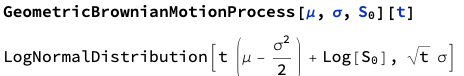
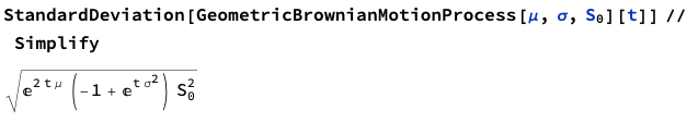
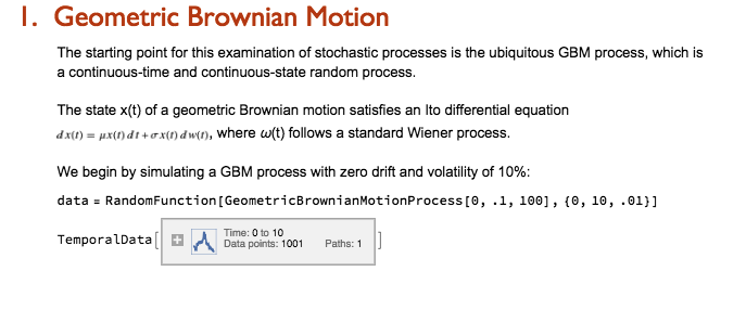
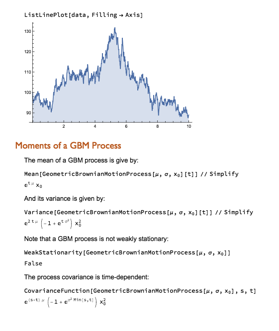
One of the most powerful aspects of the Wolfram Language is its unparalleled symbolic manipulation abilities for mathematical computation. Operations like symbolic integration, solving equations analytically, theorem proving, model simplification and more are built deeply into the language in a way no other programming language matches. Python can conduct numeric computation and data analysis well, but does not have this domain of symbolic capabilities natively.

For any usage involving abstract mathematical development, derivation of analytical results, or formal proofs, the symbolic nature of the Wolfram Language is a major differentiator.


Wolfram Notebooks

offer notable advantages over Jupyter notebooks in Python:

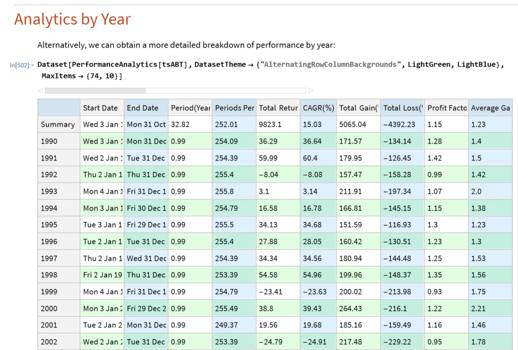
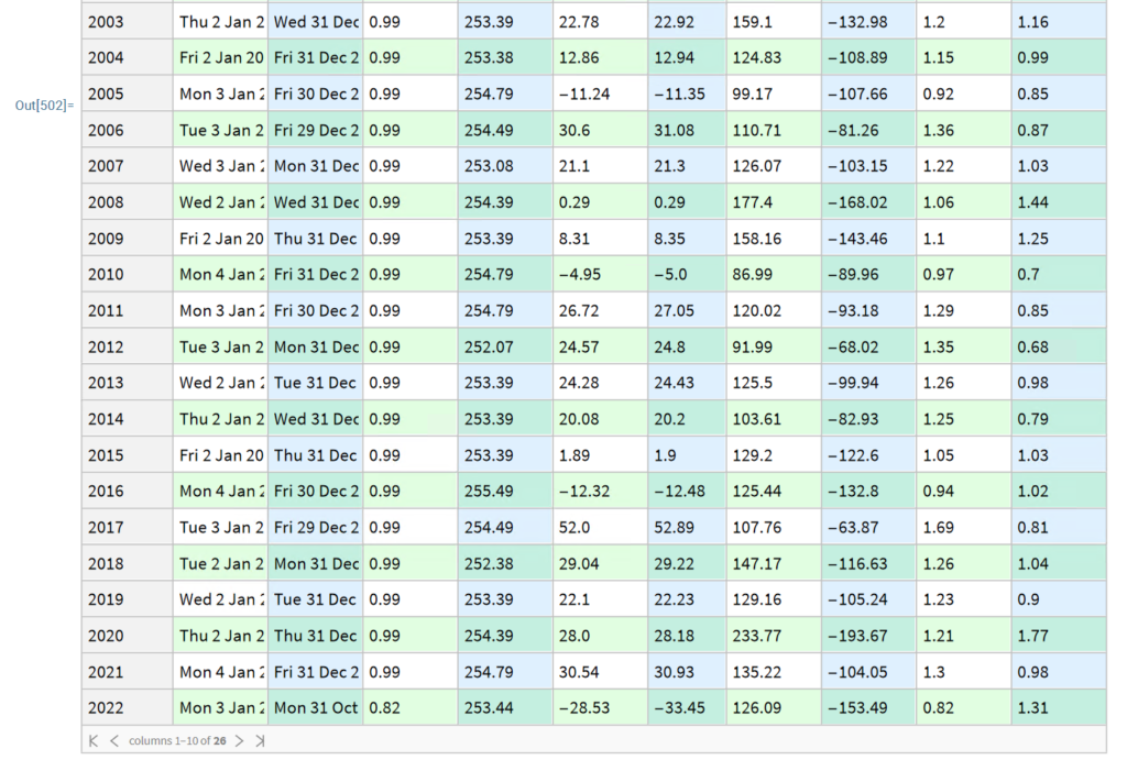
  • More visual appeal – The Wolfram notebooks produce beautifully typeset output and publication-ready visualizations by default, whereas Jupyter’s output is more basic.
  • Greater configurability – Wolfram’s notebooks allow extensive styling, templating, and customization of content for different applications. Jupyter also enables some configuration, but not to the same degree.
  • Tighter integration – The Wolfram notebooks leverage the language’s underlying functions and capabilities more fluidly since it’s one integrated environment. Jupyter interfaces well with Python but there is still some separation.
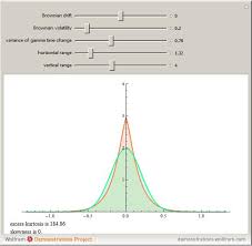
  • Interactivity – Wolfram notebooks support advanced interactivity through Manipulate/Animate and instant visual output.

    Overall, while Jupyter notebooks are hugely popular among Python developers and enable great functionality, Wolfram’s notebook solution stands out as more robust, customizable, and visually polished. The tight integration with the Wolfram Language and computational capabilities augments interactive analysis in a way Jupyter can’t match.

Integrated Knowledge and Data

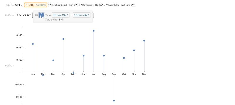
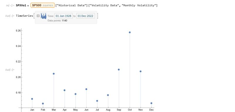
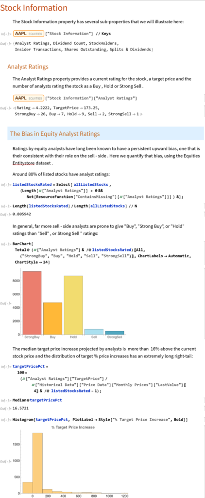
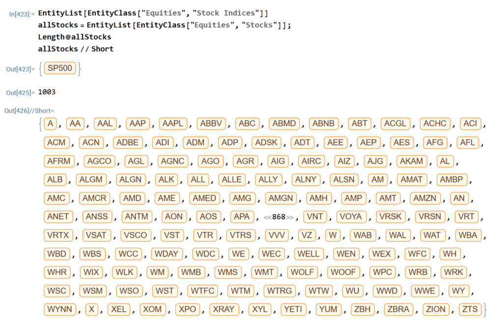
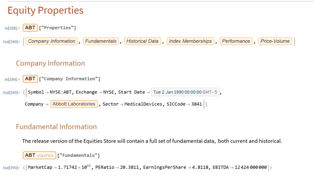
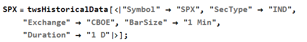
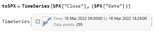
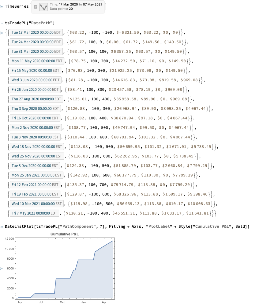
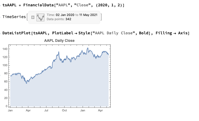
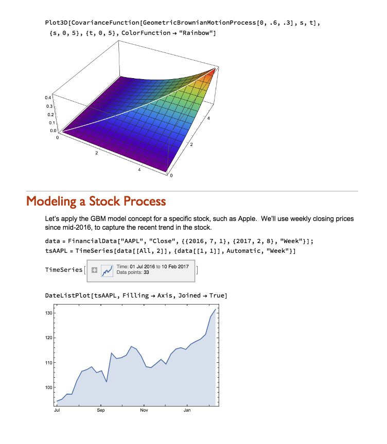
The Wolfram Language stands out in providing an “integrated knowledge base” that spans from sophisticated algorithms to real-world data across domains. This includes vast curated datasets on topics from architecture to chemistry to finance that can readily feed models and analyses without additional wrangling.

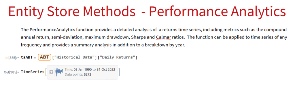
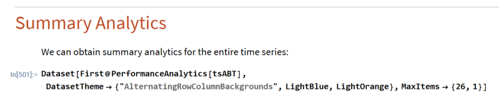
Additionally, the entity store concept allows users to author their own object-based, customizable data repositories. Python’s classes are focused on methods rather than data and while Python offers strong libraries for storing and accessing data, Wolfram facilitates more zero-friction application of real-world knowledge and entity-oriented data storage out-of-the-box. For minimizing time manipulating data or searching for reference algorithms before modeling, Wolfram Language excels.

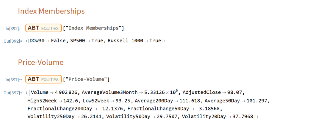
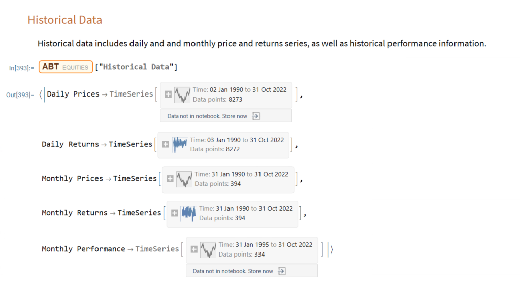
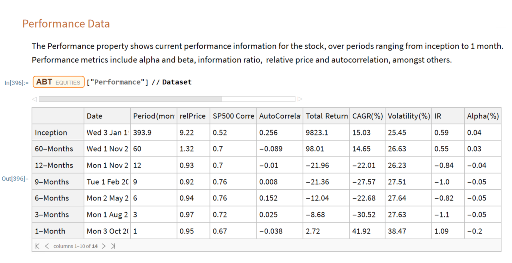
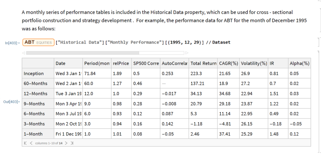
The entity store in particular enables a very natural object/entity-based programming style that can integrate smoothly with Wolfram’s class system and its underlying symbolic capabilities. This unique data representation system differentiation is a key strength (for example, see the Equities Entity Store).

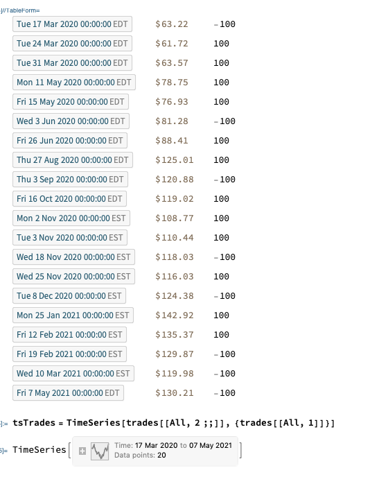
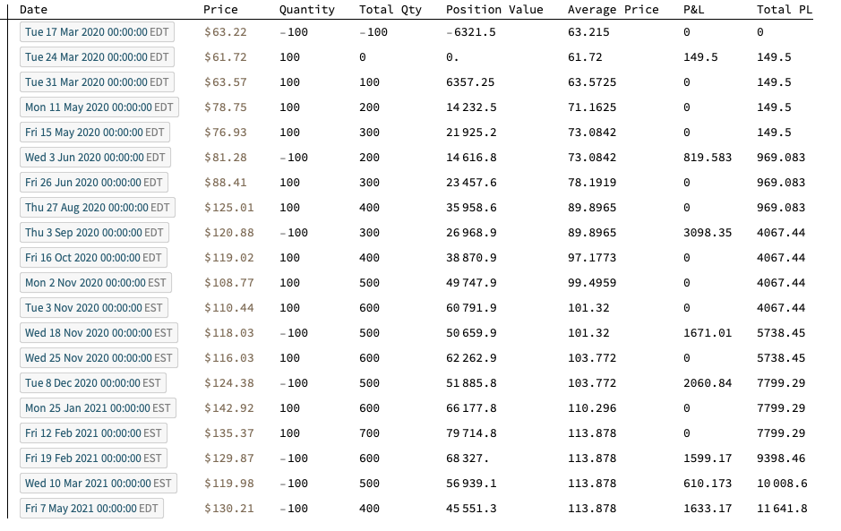
Interactivity and Prototyping

The Wolfram Language excels in hands-on analysis and rapid iteration thanks to its line-by-line execution and built-in Manipulate/Animate functions for customizable graphics, animations and interactive simulations. Python does allow some interactivity in Jupyter notebooks, but does not match Wolfram’s capabilities for creating interactive visualizations on-the-fly. This makes Wolfram Language uniquely well-suited for highly iterative, prototyping tasks that involve visual output. If ease of exploration and fluid development is a priority, the Wolfram Language has clear strengths.

Seamless Parallelization

The Wolfram Language has seamless built-in parallelization capabilities that allow code to efficiently utilize multi-core systems without the developer needing to directly manage threads or processes. Python can achieve parallelism through libraries, but the developer bears responsibility for managing dependencies and avoiding conflicts. Similarly, the Wolfram Language directly interfaces with Nvidia GPUs out-of-the-box for high performance numerical code with minimal extra effort. Thus, for users focused on computational speedup, Wolfram simplifies parallelization and GPU integration in very useful ways.

Python libraries like TensorFlow and PyTorch do hide GPU complexities well for deep learning. But in general, achieving parallel execution in Python places a greater burden on the developer. Wolfram’s approach dramatically lowers the barriers to leveraging multiple cores and GPU power for everyday computations.

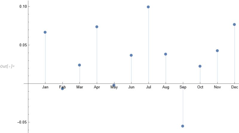
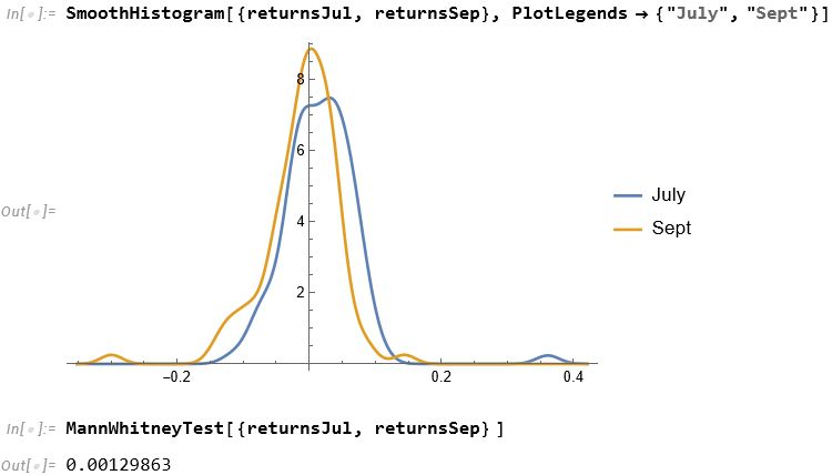
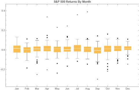
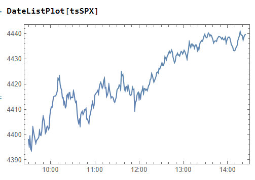
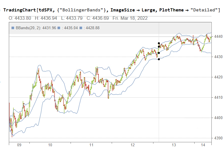
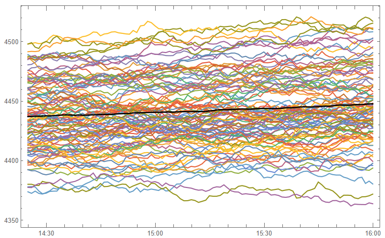
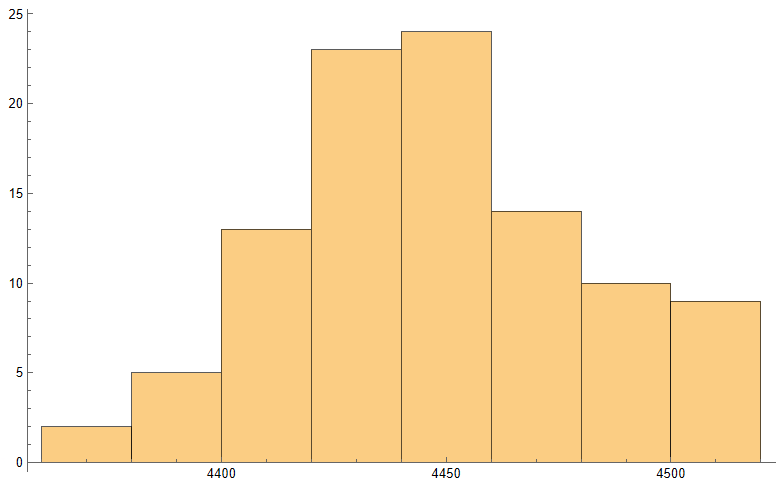
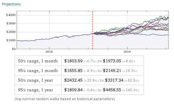
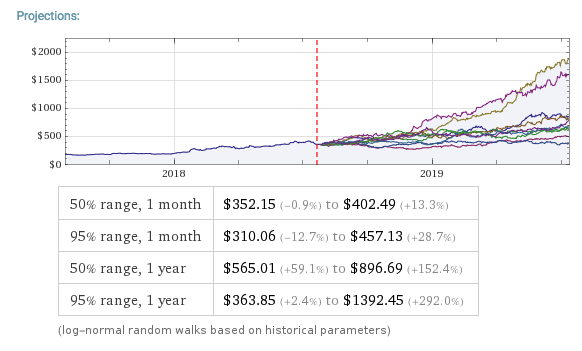
Sophisticated Visualization

Creating publication-quality, customized visualizations requires just lines of code in the Wolfram Language, thanks to the built-in graphics capabilities. While Python offers powerful visualization through add-on libraries like Matplotlib, Seaborn, Bokeh, and Plotly, Wolfram’s out-of-the-box solutions may provide greater ease of use. However, from low-level control to interactive web plots, Python’s visualization options are quite extensive despite requiring more setup. Ultimately, for rapid high-level plotting, Wolfram Language has advantageous default capabilities. But Python gives more flexibility and customization options through its ecosystem of graphic libraries.

In summary, while Python offers flexibility and a large user base – advantages in its own right – the Wolfram Language dramatically reduces lines of code and development time. By curating real-world data, algorithms, and visualization in one coherent language and platform, it streamlines and accelerates quantitative work for scientists, analysts, economists and more.

If you do significant data analysis or modeling, I encourage you to try the Wolfram Language and see the difference yourself. It’s been a gamechanger for my productivity.

Seasonality in Equity Returns

To amplify Valérie Noël‘s post a little, we can use the Equities Entity Store (https://lnkd.in/epg-5wwM) to extract returns for the S&P500 index for (almost) the last century and compute the average return by month, as follows.

July is shown to be (by far) the most positive month for the index, with an average return of +1.67%, in stark contrast to the month of Sept. in which the index has experienced an average negative return of -1.15%.

Continuing the analysis a little further, we can again use the the Equities Entity Store (https://lnkd.in/epg-5wwM) to extract estimated average volatility for the S&P500 by calendar month since 1927:

As you can see, July is not only the month with highest average monthly return, but also has amongst the lowest levels of volatility, on average.

Consequently, risk-adjusted average rates of return in July far exceed other months of the year.

Conclusion: bears certainly have a case that the market is over-stretched here, but I would urge caution: hold off until end Q3 before shorting this market in significant size.

For those market analysts who prefer a little more analytical meat, we can compare the median returns for the #S&P500 Index for the months of July and September using the nonparametric MannWhitney test.

This indicates that there is only a 0.13% probability that the series of returns for the two months are generated from distributions with the same median.

Conclusion: Index performance in July really is much better than in September.

For more analysis along these lines, see my recent book, Equity Analytics:

Equity Analytics in the Equities Data Store

Equities Entity Store  – A Brief Review

The Equities Entity Store applies the object-oriented concept of Entity Stores in the Wolfram Language to create a collection of equity objects, both stocks and stock indices, containing current and historical fundamental, technical and performance-related data. Also included in the release version of the product will be a collection of utility functions (a.k.a. “Methods”) that will facilitate equity analysis,  the formation and evaluation of equity portfolios and the development and back-testing of equities strategies, including cross-sectional strategies.

In the pre-release version of the store there are just over 1,000 equities, but this will rise to over 2,000 in the first release, as delisted securities are added to the store. This is important in order to eliminate survivor bias from the data set.

First Release of the Equities Entity Store – January 2023

The first release of the equities entity store product will contain around 2,000-2,500 equities, including at least 1,000 active stocks listed on the NYSE and NASDAQ exchanges and a further 1,000-1,500 delisted securities. All of the above information will be available for each equity and, in addition, the historical data will include quarterly fundamental data.

The other major component of the store will be analytics tools, including single-stock analytics functions such as those illustrated here. More important, however, is that the store will contain advanced analytics tools designed to assist the analyst in the construction of optimized equity portfolios and in the development and backtesting of long and long/short equity strategies.

Readers wishing to receive more information should contact me at algosciences (at) gmail.com

Intraday Stock Index Forecasting

In a previous post I discussed modelling stock prices processes as Geometric brownian Motion processes:

Understanding Stock Price Range Forecasts

To recap briefly, we assume a process of the form:

Where S0 is the initial stock price at time t = 0.

The mean of such a process is:

and standard deviation:

In the post I showed how to estimate such a process with daily stock prices, using these to provide a forecast range of prices over a one-month horizon. This is potentially useful, for example, in choosing which strikes to select in an option hedge.

Of course, there is nothing to prevent you from using the same technique over different timescales. Here I use the MATH-TWS package to connect Mathematica to the IB TWS platform via the C++ api, to extract intraday prices for the S&P 500 Index at 1-minute intervals. These are used to estimate a short-term GBM process, which provides forecasts of the mean and variance of the index at the 4 PM close.

We capture the data using:

then create a time series of the intraday prices and plot them:

If we want something a little fancier we can create a trading chart, including technical indicators of our choice, for instance:

The charts can be updated in real time from IB, using MATHTWS.

From there we estimate a GBM process using 1-minute close prices:

and then simulate a number of price paths towards the 4 PM close (the mean price path is shown in black):

This indicates that the expected value of the SPX index at the close will be around 4450, which we could estimate directly from:

Where u is the estimated drift of the GBM process.

Similarly we can look at the projected terminal distribution of the index at 4pm to get a sense of the likely range of closing prices, which may assist a decision to open or close certain option (hedge) positions:

Of course, all this is predicated on the underlying process continuing on its current trajectory, with drift and standard deviation close to those seen in the process in the preceding time interval. But trends change, as do volatilities, which means that our forecasts may be inaccurate. Furthermore, the drift in asset processes tends to be dominated by volatility, especially at short time horizons.

So the best way to think of this is as a conditional expectation, i.e. “If the stock price continues on its current trajectory, then our expectation is that the closing price will be in the following range…”.

For more on MATH-TWS see:

MATH-TWS: Connecting Wolfram Mathematica to IB TWS

Strategy Backtesting in Mathematica

This is a snippet from a strategy backtesting system that I am currently building in Mathematica.

One of the challenges when building systems in WL is to avoid looping wherever possible. This can usually be accomplished with some thought, and the efficiency gains can be significant. But it can be challenging to get one’s head around the appropriate construct using functions like FoldList, etc, especially as there are often edge cases to be taken into consideration.

A case in point is the issue of calculating the profit and loss from individual trades in a trading strategy. The starting point is to come up with a FoldList compatible function that does the necessary calculations:

CalculateRealizedTradePL[{totalQty_, totalValue_, avgPrice_, PL_,
totalPL_}, {qprice_, qty_}] :=
Module[{newTotalPL = totalPL, price = QuantityMagnitude[qprice],
newTotalQty, tradeValue, newavgPrice, newTotalValue, newPL},
newTotalQty = totalQty + qty;
tradeValue =
If[Sign[qty] == Sign[totalQty] || avgPrice == 0, priceqty, If[Sign[totalQty + qty] == Sign[totalQty], avgPriceqty,
price(totalQty + qty)]]; newTotalValue = If[Sign[totalQty] == Sign[newTotalQty], totalValue + tradeValue, newTotalQtyprice];
newavgPrice =
If[Sign[totalQty + qty] ==
Sign[totalQty], (totalQtyavgPrice + tradeValue)/newTotalQty, price]; newPL = If[(Sign[qty] == Sign[totalQty] ) || totalQty == 0, 0, qty(avgPrice - price)];
newTotalPL = newTotalPL + newPL;
{newTotalQty, newTotalValue, newavgPrice, newPL, newTotalPL}]

Trade P&L is calculated on an average cost basis, as opposed to FIFO or LIFO.

Note that the functions handle both regular long-only trading strategies and short-sale strategies, in which (in the case of equities), we have to borrow the underlying stock to sell it short. Also, the pointValue argument enables us to apply the functions to trades in instruments such as futures for which, unlike stocks, the value of a 1 point move is typically larger than 1(e.g.50 for the ES S&P 500 mini futures contract).

We then apply the function in two flavors, to accommodate both standard numerical arrays and timeseries (associations would be another good alternative):

CalculateRealizedPLFromTrades[tradeList_?ArrayQ, pointValue_ : 1] :=
Module[{tradePL =
Rest@FoldList[CalculateRealizedTradePL, {0, 0, 0, 0, 0},
tradeList]},
tradePL[[All, 4 ;; 5]] = tradePL[[All, 4 ;; 5]]pointValue; tradePL] CalculateRealizedPLFromTrades[tsTradeList_, pointValue_ : 1] := Module[{tsTradePL = Rest@FoldList[CalculateRealizedTradePL, {0, 0, 0, 0, 0}, QuantityMagnitude@tsTradeList["Values"]]}, tsTradePL[[All, 4 ;; 5]] = tsTradePL[[All, 4 ;; 5]]pointValue;
tsTradePL[[All, 2 ;;]] =
Quantity[tsTradePL[[All, 2 ;;]], "US Dollars"];
tsTradePL =
TimeSeries[
Transpose@
Join[Transpose@tsTradeList["Values"], Transpose@tsTradePL],
tsTradeList["DateList"]]]

These functions run around 10x faster that the equivalent functions that use Do loops (without parallelization or compilation, admittedly).

Let’s see how they work with an example:

Trade Simulation

Next, we’ll generate a series of random trades using the AAPL time series, as follows (we also take the opportunity to convert the list of trades into a time series, tsTrades):

trades = Transpose@
Join[Transpose[
tsAAPL["DatePath"][[
Sort@RandomSample[Range[tsAAPL["PathLength"]],
20]]]], {RandomChoice[{-100, 100}, 20]}];
trades // TableForm

Trade P&L Calculation

We are now ready to apply our Trade P&L calculation function, first to the list of trades in array form:

TableForm[
Flatten[#] & /@ 
Partition[
Riffle[trades, 
CalculateRealizedPLFromTrades[trades[[All, 2 ;; 3]]]], 2], 
TableHeadings -> {{}, {"Date", "Price", "Quantity", "Total Qty", 
"Position Value", "Average Price", "P&L", "Total PL"}}]

The timeseries version of the function provides the output as a timeseries object in Quantity[“US Dollars”] format and, of course, can be plotted immediately with DateListPlot (it is also convenient for other reasons, as the complete backtest system is built around timeseries objects):

tsTradePL = CalculateRealizedPLFromTrades[tsTrades]

Understanding Stock Price Range Forecasts

Stock Price Range Forecasts

Range forecasts are produced by estimating the parameters of a Geometric Brownian Motion process from historical data and using the model to project a large number of sample paths for the stock price over the coming month and year.

For example, this is a range forecast for Netflix, Inc. (NFLX) as at 7/27/2018 when the price of the stock stood at $355.21:

$NFLX

As you can see, the great majority of the simulated price paths trend upwards.  This is typical for most stocks on account of their upward drift, a tendency to move higher over time.  The statistical table below the chart tells you that in 50% of cases the ending stock price 1 month from the date of forecast was in the range $352.15 to $402.49. Similarly, around 50% of the time the price of the stock in one year’s time were found to be in the range $565.01 to $896.69.  Notice that the end points of the one-year range far exceed the end points of the one-month range forecast – again this is a feature of the upward drift in stocks.

If you want much greater certainty about the outcome, you should look at the 95% ranges.  So, for NFLX, the one month 95% range was projected to be $310.06 to $457.13.  Here, only 1 in 20 of the simulated price paths produced one month forecasts that were higher than $457.13, or lower than $310.06.

Notice that the spread of the one month and one year 95% ranges is much larger than of the corresponding 50% ranges.  This demonstrates the fundamental tradeoff between “accuracy” (the spread of the range) and “certainty”, (the probability of the outcome being with the projected range).  If you want greater certainty of the outcome, you have to allow for a broader span of possibilities, i.e. a wider range.

SSALGOTRADING AD

Uses of Range Forecasts

Most stock analysts tend to produce single price “targets”, rather than a range – these are known as “point forecasts” by econometricians.  So what’s the thinking behind range forecasts?

Range forecasts are arguably more useful than simple point forecasts.  Point forecasts make no guarantee as to the likelihood of the projected price – the only thing we know for sure about such forecasts is that they will be wrong!  Is the forecast target price optimistic or pessimistic?  We have no way to tell.

With range forecasts the situation is very different.  We can talk about the likelihood of a stock being within a specified range at a certain point in time.  If we want to provide a pessimistic forecast for the price in NFLX in one month’s time, for example, we could quote the value $352.15, the lower end of the 50% range forecast.  If we wanted to provide a very pessimistic forecast, one that is very likely to be exceeded, we could quote the bottom of the 95% range: $310.06.

The range also tells us about the future growth prospects for the firm.  So, for example, with NFLX, based on past performance, it is highly likely that the stock price will grow at a rate of more than 2.4% and, optimistically, might increase by almost 3x in the coming year (see the growth rates calculated for the 95% range values).

One specific use of range forecasts is in options trading.  If a trader is bullish on NFLX, instead of buying the stock, he might instead choose to sell one-month put options with a strike price below $352 (the lower end of the 50% one-month range).  If the trader wanted to be more conservative, he might look for put options struck at around $310, the bottom of the 95% range.  A more complex strategy might be to buy calls struck near the top of the 50% range, and sell more calls struck near the top of the 95% range (the theory being that the stock is quite likely to exceed the top of the 50% one-month range, but much less likely to reach the high end of the 95% range).

Limitations of Range Forecasts

Range forecasts are produced by using historical data to estimate the parameters of a particular type of mathematical model, known as a Geometric Brownian Motion process.  For those who are interested in the mechanics of how the forecasts are produced, I have summarized the relevant background theory below.

While there are grounds for challenging the use of such models in this context, it has to be acknowledged that the GBM process is one of the most successful mathematical models in finance today.  The problem lies not so much in the model, as in one of the key assumptions underpinning the approach:  specifically, that the characteristics of the stock process will remain as they are today (and as they have been in the historical past).  This assumption is manifestly untenable when applied to many stocks:  a company that was a high-growth $100M start-up is unlikely to demonstrate the same  rate of growth ten years later, as a $10Bn enterprise.  A company like Amazon that started out as an online book seller has fundamentally different characteristics today, as an online retail empire.  In such cases, forecasts about the future stock price – whether point or range forecasts – based on outdated historical informations are likely to be wrong, sometimes wildly so.

Having said that, there are a great many companies that have evolved to a point of relative stability over a period of perhaps several decades: for example, a company like Caterpillar Inc. (CAT).  In such cases the parameters of the GBM process underpinning the stock price are unlikely to fluctuate widely in the short term, so range forecasts are consequently more likely to be useful.

Another factor to consider are quarterly earnings reports, which can influence stock prices considerably in the short term, and corporate actions (mergers, takeovers, etc) that can change the long term characteristics of a firm and its stock price process in a fundamental way.  In these situations any forecast methodology is likely to unreliable, at least for a while, until the event has passed.  It’s best to avoid taking positions based on projections from historical data at times like this.

Review of Background Theory


GBM1

GBM2 GBM3 GBM4 GBM5