Machine Learning Trading Systems

The SPDR S&P 500 ETF (SPY) is one of the widely traded ETF products on the market, with around $200Bn in assets and average turnover of just under 200M shares daily.  So the likelihood of being able to develop a money-making trading system using publicly available information might appear to be slim-to-none. So, to give ourselves a fighting chance, we will focus on an attempt to predict the overnight movement in SPY, using data from the prior day’s session.

In addition to the open/high/low and close prices of the preceding day session, we have selected a number of other plausible variables to build out the feature vector we are going to use in our machine learning model:

  • The daily volume
  • The previous day’s closing price
  • The 200-day, 50-day and 10-day moving averages of the closing price
  • The 252-day high and low prices of the SPY series

We will attempt to build a model that forecasts the overnight return in the ETF, i.e.  [O(t+1)-C(t)] / C(t)

SSALGOTRADING AD

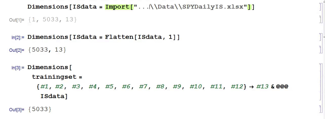
In this exercise we use daily data from the beginning of the SPY series up until the end of 2014 to build the model, which we will then test on out-of-sample data running from Jan 2015-Aug 2016.  In a high frequency context a considerable amount of time would be spent evaluating, cleaning and normalizing the data.  Here we face far fewer problems of that kind.  Typically one would standardized the input data to equalize the influence of variables that may be measured on scales of very different orders of magnitude.  But in this example all of the input variables, with the exception of volume, are measured on the same scale and so standardization is arguably unnecessary.

First, the in-sample data is loaded and used to create a training set of rules that map the feature vector to the variable of interest, the overnight return:


fig1


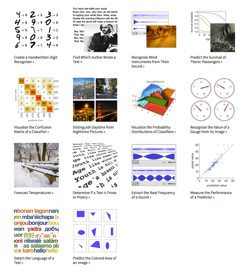
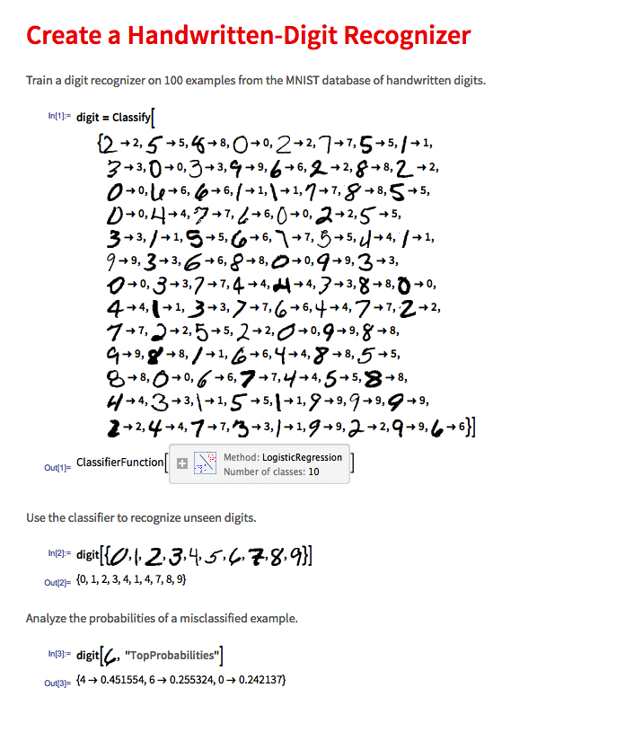
In Mathematica 10 Wolfram introduced a suite of machine learning algorithms that include regression, nearest neighbor, neural networks and random forests, together with functionality to evaluate and select the best performing machine learning technique.  These facilities make it very straightfoward to create a classifier or prediction model using machine learning algorithms, such as this handwriting recognition example:

handwriting

We create a predictive model on the SPY trainingset, allowing Mathematica to pick the best machine learning algorithm:

fig3

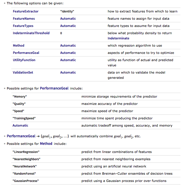
There are a number of options for the Predict function that can be used to control the feature selection, algorithm type, performance type and goal, rather than simply accepting the defaults, as we have done here:

fig4

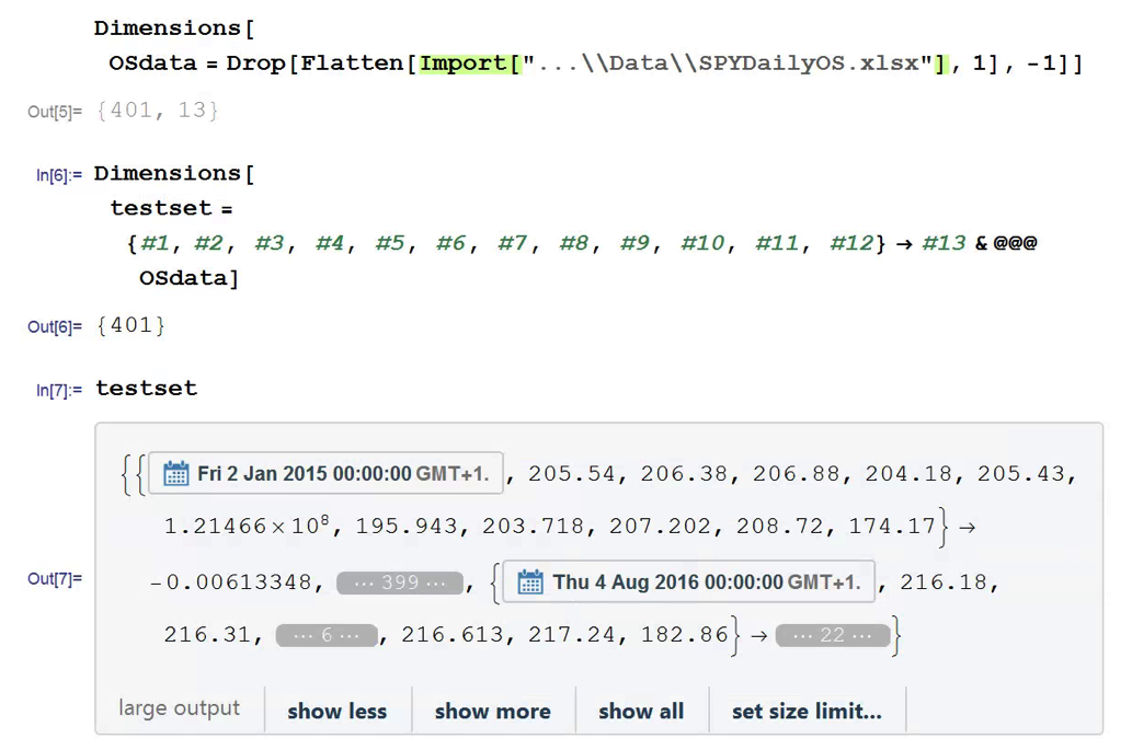
Having built our machine learning model, we load the out-of-sample data from Jan 2015 to Aug 2016, and create a test set:

fig5


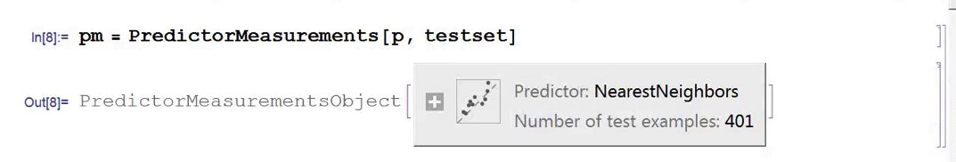
We next create a PredictionMeasurement object,  using the Nearest Neighbor model , that can be used for further analysis:


fig6

fig7

fig8


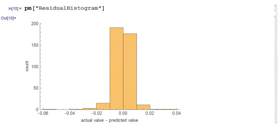
There isn’t much dispersion in the model forecasts, which all have positive value.  A common technique in such cases is to subtract the mean from each of the forecasts (and we may also standardize them by dividing by the standard deviation).

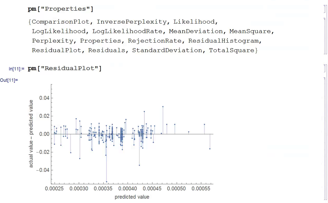
The scatterplot of actual vs. forecast overnight returns in SPY now looks like this:

scatterplot


There’s still an obvious lack of dispersion in the forecast values, compared to the actual overnight returns, which we could rectify by standardization. In any event, there appears to be a small, nonlinear relationship between forecast and actual values, which holds out some hope that the model may yet prove useful.

From Forecasting to Trading

There are various methods of deploying a forecasting model in the context of creating a trading system.  The simplest route, which we  will take here, is to apply a threshold gate and convert the filtered forecasts directly into a trading signal. But other approaches are possible, for example:

  • Combining the forecasts from multiple models to create a prediction ensemble
  • Using the forecasts as inputs to a genetic programming model
  • Feeding the forecasts into the input layer of  a neural network model designed specifically to generate trading signals, rather than forecasts

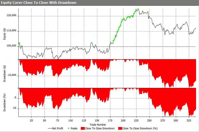
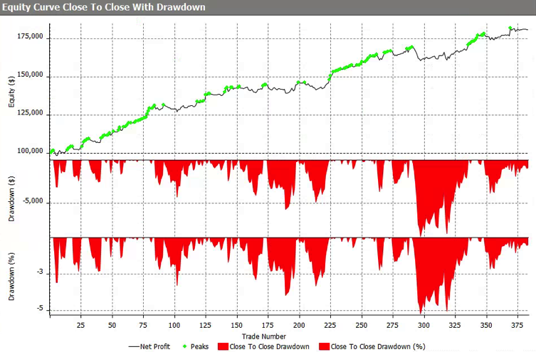
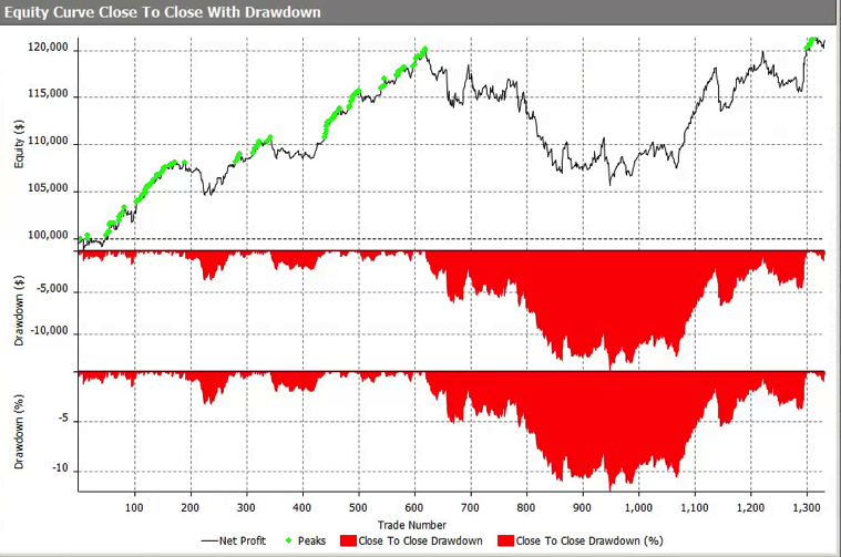
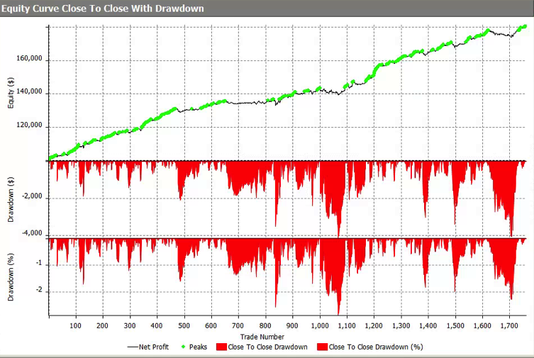
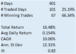
In this example we will create a trading model by applying a simple filter to the forecasts, picking out only those values that exceed a specified threshold. This is a standard trick used to isolate the signal in the model from the background noise.  We will accept only the positive signals that exceed the threshold level, creating a long-only trading system.  i.e. we ignore forecasts that fall below the threshold level.  We buy SPY at the close when the forecast exceeds the threshold and exit any long position at the next day’s open.  This strategy produces the following pro-forma results:


Perf table


equity curve


Conclusion

The system has some quite attractive features, including a win rate of over 66%  and a CAGR of over 10% for the out-of-sample period.

Obviously, this is a very basic illustration: we would want to factor in trading commissions, and the slippage incurred entering and exiting positions in the post- and pre-market periods, which will negatively impact performance, of course.  On the other hand, we have barely begun to scratch the surface in terms of the variables that could be considered for inclusion in the feature vector, and which may increase the explanatory power of the model.

In other words, in reality, this is only the beginning of a lengthy and arduous research process. Nonetheless, this simple example should be enough to give the reader a taste of what’s involved in building a predictive trading model using machine learning algorithms.


The Information Content of the Pre- and Post-Market Trading Sessions

I apologize in advance for this rather “wonkish” post, which is aimed chiefly at the high frequency fraternity, or those at least who trade intra-day, in the equity markets.  Such minutiae are the lot of those engaged in high frequency trading.  I promise that my next post will be of more general interest.

Pre- and Post Market Sessions

The pre-market session in US equities runs from 8:00 AM ET, while the post-market session runs until 8:00 PM ET.  The question arises whether these sessions are worth trading, or at the very least, offer a source of data (quotes, trades) that might be relevant to trading the regular session, which of course runs from 9:30 AM to 4:00 PM ET.  Even if liquidity is thin and trades infrequent, and opportunities in the pre- and post-market very limited, it might be that we can improve our trading models by taking into account such information as these sessions do provide, even if we only ever plan to trade during regular trading hours.

It is somewhat challenging to discuss this in great detail, because HFT equity trading is very much in the core competencies of my firm, Systematic Strategies.  However, I hope to offer some ideas, at least, that some readers may find useful.

SSALGOTRADING AD


A Tale of Two Pharmaceutical Stocks

In what follows I am going to make use of two examples from the pharmaceutical industry: Alexion Pharmaceuticals, Inc. (ALXN), which has a market cap of $35Bn and trades around 800,000 shares daily, and Pfizer Inc. (PFE), which has a market cap of over $200Bn and trades close to 50M shares a day.

Let’s start by looking at a system trading ALXN during regular market hours.  The system isn’t high frequency, but trades around 1-2 times a day, on average.  The strategy equity curve from 2015 to April 2016 is not at all impressive.


ALXN Regular

ALXN – Regular Session Only


But look at the equity curve for the same strategy when we allow it to run on the pre- and post-market sessions, in addition to regular trading hours.  Clearly the change in the trading hours utilized by the strategy has made a huge improvement in the total gain and risk-adjusted returns.


ALEXN with pre-market

ALXN – with Pre- and Post-Market Sessions


The PFE system trades much more frequently, around 4 times a day, but the story is somewhat similar in terms of how including the pre- and post-market sessions appears to improve its performance.

PFE Regular

PFE – Regular Session Only

PFE with premarket

PFE – with Pre- and Post-Market Sessions


Improving Trading Performance

In both cases, clearly, the trading performance of the strategies has improved significantly with the inclusion of the out-of-hours sessions.  In the case of ALXN, we see a modest increase of around 10% in the total number of trades, but in the case of PFE the increase in trading activity is much more marked – around 30%, or more.

The first important question to ask is when these additional trades are occurring.  Assuming that most of them take place during the pre- or post-market, our concern might be whether there is likely to be sufficient liquidity to facilitate trades of the frequency and size we wish to execute.  Of various possible hypotheses, some negative, other positive, we might consider the following:

(a) Bad ticks in the market data feed during out-of-hours sessions give rise to apparently highly profitable “phantom” trades

(b) The market data is valid, but the trades are done in such low volume as to be insignificant for practical purposes (i.e. trades were done for a few hundred lots and additional liquidity is unlikely to be available)

(c) Out-of-hours sessions enable the system to improve profitability by entering or exiting positions in a more timely manner than by trading the regular session alone

(d) Out-of-hours market data improves the accuracy of model forecasts, facilitating a larger number of trades, and/or more profitable trades, during regular market hours

An analysis of the trading activity for the two systems provides important insight as to which of the possible explanations might be correct.


ALXN Analysis

(click to enlarge)

Dealing first with ALXN, we that, indeed, an additional 11% of trades are entered or exited out-of-hours.  However, these additional trades account for somewhere between 17% (on exit) and 20% (on entry) of the total profits.  Furthermore, the size of the average entry trade during the post-market session and of the average exit trade in the pre-market session is more than double that of the average trade entered or exited during regular market hours. That gives concerns that some of the apparent increase in profits may be due to bad ticks at prices away from the market, allowing the system enter or exit trades at unrealistically low or high prices.  Even if many of the trades are good, we will have concerns about the scalability of the strategy in out-of-hours trading, given the relatively poor liquidity in the stock. On the other hand, at least some of the uplift in profits arises from new trades occurring during the regular session. This suggests that, even if we are unable to execute many of the trading opportunities seen during pre- or post-market, the trades from those sessions provides useful additional data points for our model, enabling it to increase the number and/or profitability of trades in the regular session.

Next we turn to PFE.  We can see straight away that, while the proportion of trades occurring during out-of-hours sessions is around 23%, those trades now account for over 50% of the total profits.  Furthermore, the average PL for trades executed on entry post-market, and on exit pre-market, is more than 4x the average for trades entered or exited during normal market hours.  Despite the much better liquidity in PFE compared to ALXN, this is a huge concern – we might expect to see significant discrepancies occurring between theoretical and actual performance of the strategy, due to the very high dependency on out-of-hours trading.

PFE Analysis

(click to enlarge)

As we dig further into the analysis, we do indeed find evidence that bad data ticks play a disproportionate role.  For example, this trade in PFE which apparently occurred at around 16:10 on 4/6 was almost certainly a phantom trade resulting from a bad data point. It turns out that, for whatever reason, such bad ticks are a common occurrence in the stock and account for a large proportion of the apparent profitability of out-of-hours trading in PFE.


PFE trade


CONCLUSION

We are, of course, only skimming the surface of the analysis that is typically carried out.  One would want to dig more deeply into ways in which the market data feed could be cleaned up and bad data ticks filtered out so as to generate fewer phantom trades.  One would also want to look at liquidity across the various venues where the stocks trade, including dark pools, in order to appraise the scalability of the strategies.

For now, the main message that I am seeking to communicate is that it is often well worthwhile considering trading in the pre- and post-market sessions, not only with a view to generating additional, profitable trading opportunities, but also to gather additional data points that can enhance trading profitability during regular market hours.