
Trading Anomalies

An extract from my new book, Equity Analytics.
Trading-Anomalies-2Statistical Arbitrage with Synthetic Data

In my last post I mapped out how one could test the reliability of a single stock strategy (for the S&P 500 Index) using synthetic data generated by the new algorithm I developed.
As this piece of research follows a similar path, I won’t repeat all those details here. The key point addressed in this post is that not only are we able to generate consistent open/high/low/close prices for individual stocks, we can do so in a way that preserves the correlations between related securities. In other words, the algorithm not only replicates the time series properties of individual stocks, but also the cross-sectional relationships between them. This has important applications for the development of portfolio strategies and portfolio risk management.
KO-PEP Pair
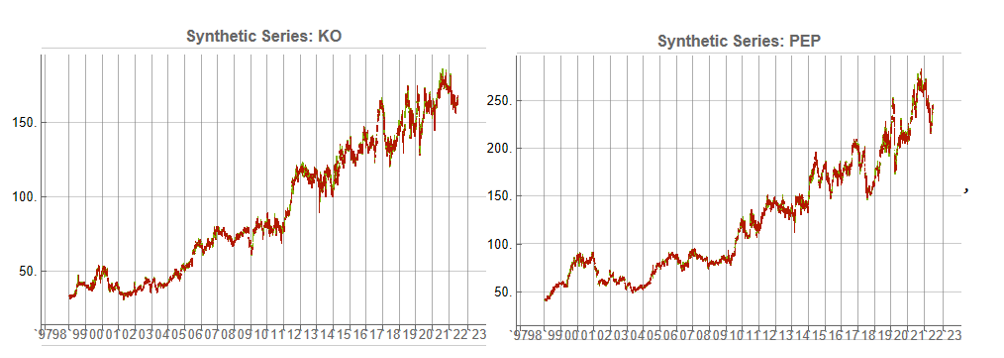
To illustrate this I will use synthetic daily data to develop a pairs trading strategy for the KO-PEP pair.
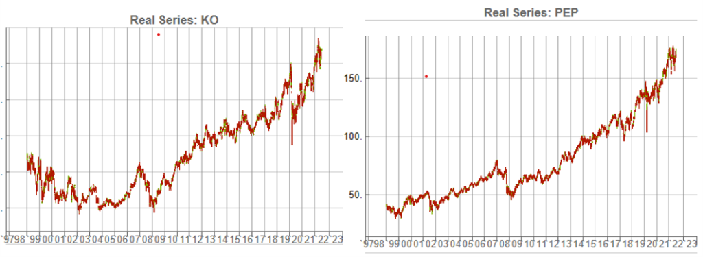
The two price series are highly correlated, which potentially makes them a suitable candidate for a pairs trading strategy.
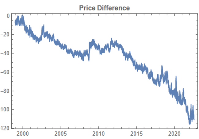
There are numerous ways to trade a pairs spread such as dollar neutral or beta neutral, but in this example I am simply going to look at trading the price difference. This is not a true market neutral approach, nor is the price difference reliably stationary. However, it will serve the purpose of illustrating the methodology.
Obviously it is crucial that the synthetic series we create behave in a way that replicates the relationship between the two stocks, so that we can use it for strategy development and testing. Ideally we would like to see high correlations between the synthetic and original price series as well as between the pairs of synthetic price data.
We begin by using the algorithm to generate 100 synthetic daily price series for KO and PEP and examine their properties.
Correlations
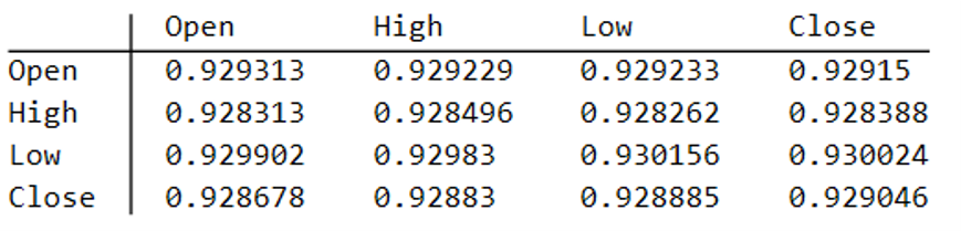
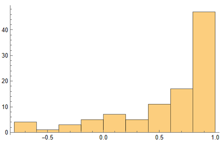
As we saw previously, the algorithm is able to generate synthetic data with correlations to the real price series ranging from below zero to close to 1.0:
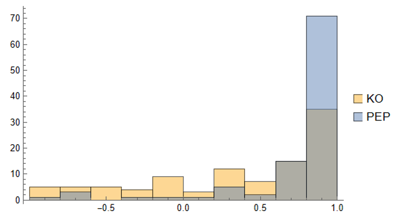
The crucial point, however, is that the algorithm has been designed to also preserve the cross-sectional correlation between the pairs of synthetic KO-PEP data, just as in the real data series:
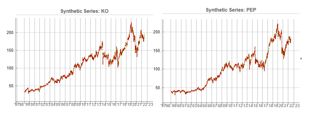
Some examples of highly correlated pairs of synthetic data are shown in the plots below:
In addition to correlation, we might also want to consider the price differences between the pairs of synthetic series, since the strategy will be trading that price difference, in the simple approach adopted here. We could, for example, select synthetic pairs for which the divergence in the price difference does not become too large, on the assumption that the series difference is stationary. While that approach might well be reasonable in other situations, here an assumption of stationarity would be perhaps closer to wishful thinking than reality. Instead we can use of selection of synthetic pairs with high levels of cross-correlation, as we all high levels of correlation with the real price data. We can also select for high correlation between the price differences for the real and synthetic price series.
Strategy Development & WFO Testing
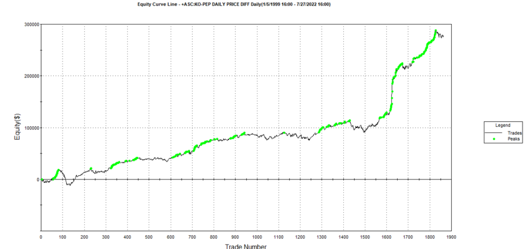
Once again we follow the procedure for strategy development outline in the previous post, except that, in addition to a selection of synthetic price difference series we also include 14-day correlations between the pairs. We use synthetic daily synthetic data from 1999 to 2012 to build the strategy and use the data from 2013 onwards for testing/validation. Eventually, after 50 generations we arrive at the result shown in the figure below:
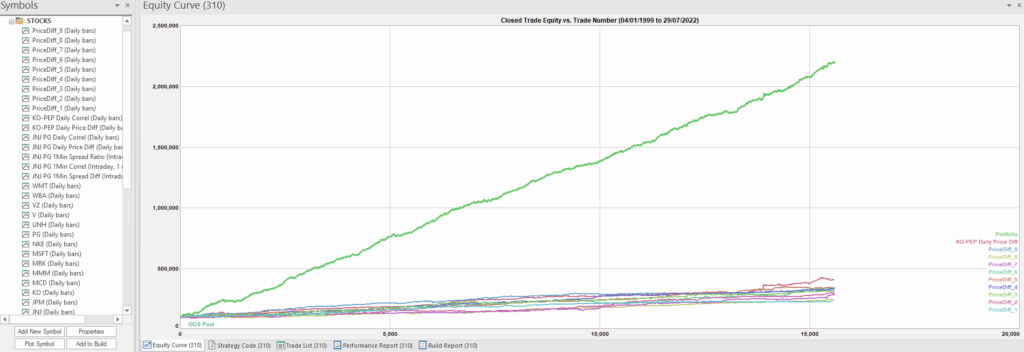
As before, the equity curve for the individual synthetic pairs are shown towards the bottom of the chart, while the aggregate equity curve, which is a composition of the results for all none synthetic pairs is shown above in green. Clearly the results appear encouraging.
As a final step we apply the WFO analysis procedure described in the previous post to test the performance of the strategy on the real data series, using a variable number in-sample and out-of-sample periods of differing size. The results of the WFO cluster test are as follows:
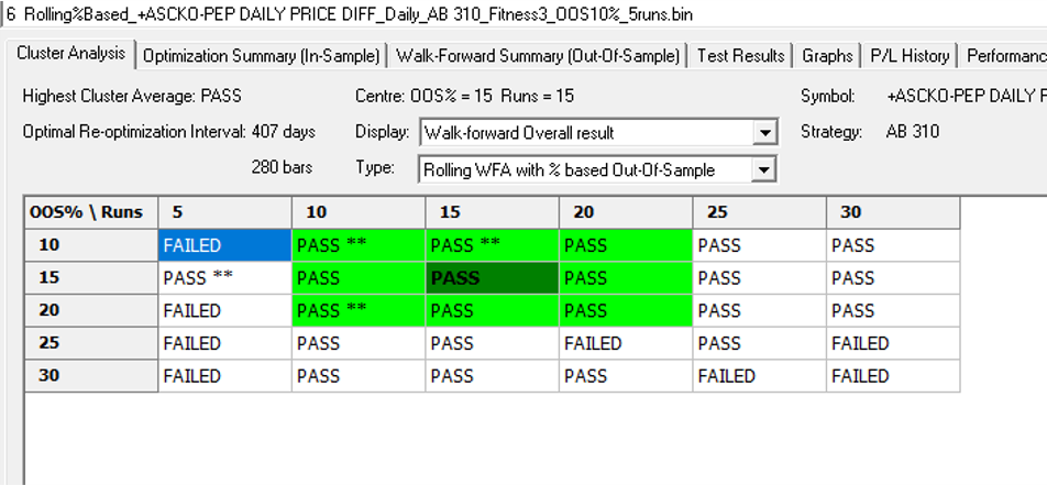
The results are no so unequivocal as for the strategy developed for the S&P 500 index, but would nonethless be regarded as acceptable, since the strategy passes the great majority of the tests (in addition to the tests on synthetic pairs data).
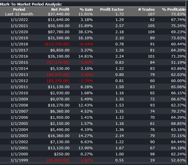
The final results appear as follows:
Conclusion
We have demonstrated how the algorithm can be used to generate synthetic price series the preserve not only the important time series properties, but also the cross-sectional properties between series for correlated securities. This important feature has applications in the development of statistical arbitrage strategies, portfolio construction methodology and in portfolio risk management.
Tactical Mutual Fund Strategies

A recent blog post of mine was posted on Seeking Alpha (see summary below if you missed it).
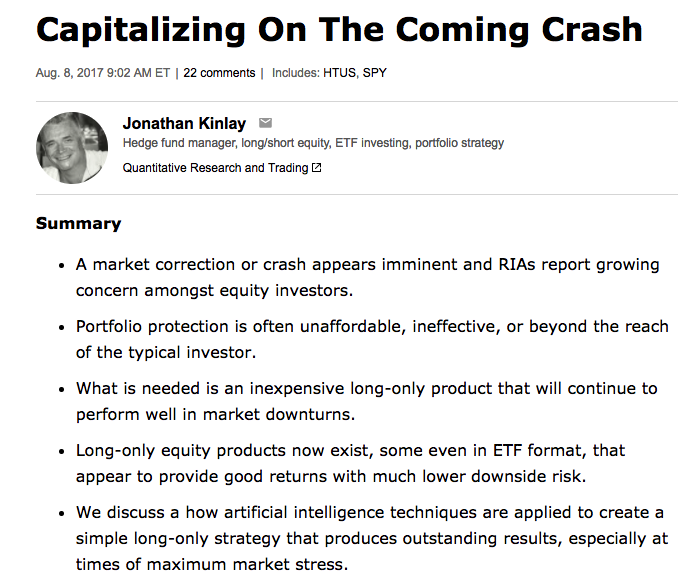
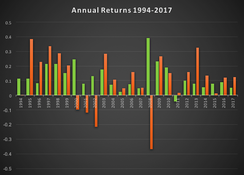
The essence of the idea is simply that one can design long-only, tactical market timing strategies that perform robustly during market downturns, or which may even be positively correlated with volatility. I used the example of a LOMT (“Long-Only Market-Timing”) strategy that switches between the SPY ETF and 91-Day T-Bills, depending on the current outlook for the market as characterized by machine learning algorithms. As I indicated in the article, the LOMT handily outperforms the buy-and-hold strategy over the period from 1994 -2017 by several hundred basis points:

Of particular note is the robustness of the LOMT strategy performance during the market crashes in 2000/01 and 2008, as well as the correction in 2015:
The Pros and Cons of Market Timing (aka “Tactical”) Strategies
One of the popular choices the investor concerned about downsize risk is to use put options (or put spreads) to hedge some of the market exposure. The problem, of course, is that the cost of the hedge acts as a drag on performance, which may be reduced by several hundred basis points annually, depending on market volatility. Trying to decide when to use option insurance and when to maintain full market exposure is just another variation on the market timing problem.
The point of tactical strategies is that, unlike an option hedge, they will continue to produce positive returns – albeit at a lower rate than the market portfolio – during periods when markets are benign, while at the same time offering much superior returns during market declines, or crashes. If the investor is concerned about the lower rate of return he is likely to achieve during normal years, the answer is to make use of leverage.

Market timing strategies like Hull Tactical or the LOMT have higher risk-adjusted rates of return (Sharpe Ratios) than the market portfolio. So the investor can make use of margin money to scale up his investment to about the same level of risk as the market index. In doing so he will expect to earn a much higher rate of return than the market.
This is easy to do with products like LOMT or Hull Tactical, because they make use of marginable securities such as ETFs. As I point out in the sections following, one of the shortcomings of applying the market timing approach to mutual funds, however, is that they are not marginable (not initially, at least), so the possibilities for using leverage are severely restricted.
Market Timing with Mutual Funds
An interesting suggestion from one Seeking Alpha reader was to apply the LOMT approach to the Vanguard 500 Index Investor fund (VFINX), which has a rather longer history than the SPY ETF. Unfortunately, I only have ready access to data from 1994, but nonetheless applied the LOMT model over that time period. This is an interesting challenge, since none of the VFINX data was used in the actual construction of the LOMT model. The fact that the VFINX series is highly correlated with SPY is not the issue – it is typically the case that strategies developed for one asset will fail when applied to a second, correlated asset. So, while it is perhaps hard to argue that the entire VFIX is out-of-sample, the performance of the strategy when applied to that series will serve to confirm (or otherwise) the robustness and general applicability of the algorithm.
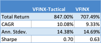
The results turn out as follows:
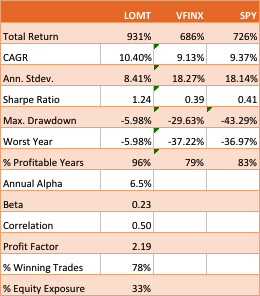
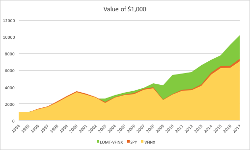
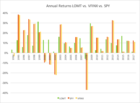
The performance of the LOMT strategy implemented for VFINX handily outperforms the buy-and-hold portfolios in the SPY ETF and VFINX mutual fund, both in terms of return (CAGR) and well as risk, since strategy volatility is less than half that of buy-and-hold. Consequently the risk adjusted return (Sharpe Ratio) is around 3x higher.
That said, the VFINX variation of LOMT is distinctly inferior to the original version implemented in the SPY ETF, for which the trading algorithm was originally designed. Of particular significance in this context is that the SPY version of the LOMT strategy produces substantial gains during the market crash of 2008, whereas the VFINX version of the market timing strategy results in a small loss for that year. More generally, the SPY-LOMT strategy has a higher Sortino Ratio than the mutual fund timing strategy, a further indication of its superior ability to manage downside risk.
Given that the objective is to design long-only strategies that perform well in market downturns, one need not pursue this particular example much further , since it is already clear that the LOMT strategy using SPY is superior in terms of risk and return characteristics to the mutual fund alternative.
Practical Limitations
There are other, practical issues with apply an algorithmic trading strategy a mutual fund product like VFINX. To begin with, the mutual fund prices series contains no open/high/low prices, or volume data, which are often used by trading algorithms. Then there are the execution issues: funds can only be purchased or sold at market prices, whereas many algorithmic trading systems use other order types to enter and exit positions (stop and limit orders being common alternatives). You can’t sell short and there are restrictions on the frequency of trading of mutual funds and penalties for early redemption. And sales loads are often substantial (3% to 5% is not uncommon), so investors have to find a broker that lists the selected funds as no-load for the strategy to make economic sense. Finally, mutual funds are often treated by the broker as ineligible for margin for an initial period (30 days, typically), which prevents the investor from leveraging his investment in the way that he do can quite easily using ETFs.
For these reasons one typically does not expect a trading strategy formulated using a stock or ETF product to transfer easily to another asset class. The fact that the SPY-LOMT strategy appears to work successfully on the VFINX mutual fund product (on paper, at least) is highly unusual and speaks to the robustness of the methodology. But one would be ill-advised to seek to implement the strategy in that way. In almost all cases a better result will be produced by developing a strategy designed for the specific asset (class) one has in mind.
A Tactical Trading Strategy for the VFINX Mutual Fund
A better outcome can possibly be achieved by developing a market timing strategy designed specifically for the VFINX mutual fund. This strategy uses only market orders to enter and exit positions and attempts to address the issue of frequent trading by applying a trading cost to simulate the fees that typically apply in such situations. The results, net of imputed fees, for the period from 1994-2017 are summarized as follows:


Overall, the CAGR of the tactical strategy is around 88 basis points higher, per annum. The risk-adjusted rate of return (Sharpe Ratio) is not as high as for the LOMT-SPY strategy, since the annual volatility is almost double. But, as I have already pointed out, there are unanswered questions about the practicality of implementing the latter for the VFINX, given that it seeks to enter trades using limit orders, which do not exist in the mutual fund world.
The performance of the tactical-VFINX strategy relative to the VFINX fund falls into three distinct periods: under-performance in the period from 1994-2002, about equal performance in the period 2003-2008, and superior relative performance in the period from 2008-2017.
Only the data from 1/19934 to 3/2008 were used in the construction of the model. Data in the period from 3/2008 to 11/2012 were used for testing, while the results for 12/2012 to 8/2017 are entirely out-of-sample. In other words, the great majority of the period of superior performance for the tactical strategy was out-of-sample. The chief reason for the improved performance of the tactical-VFINX strategy is the lower drawdown suffered during the financial crisis of 2008, compared to the benchmark VFINX fund. Using market-timing algorithms, the tactical strategy was able identify the downturn as it occurred and exit the market. This is quite impressive since, as perviously indicated, none of the data from that 2008 financial crisis was used in the construction of the model.
In his Seeking Alpha article “Alpha-Winning Stars of the Bull Market“, Brad Zigler identifies the handful of funds that have outperformed the VFINX benchmark since 2009, generating positive alpha:
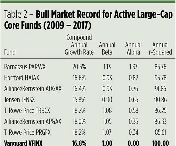
What is notable is that the annual alpha of the tactical-VINFX strategy, at 1.69%, is higher than any of those identified by Zigler as being “exceptional”. Furthermore, the annual R-squared of the tactical strategy is higher than four of the seven funds on Zigler’s All-Star list. Based on Zigler’s performance metrics, the tactical VFINX strategy would be one of the top performing active funds.
But there is another element missing from the assessment. In the analysis so far we have assumed that in periods when the tactical strategy disinvests from the VFINX fund the proceeds are simply held in cash, at zero interest. In practice, of course, we would invest any proceeds in risk-free assets such as Treasury Bills. This would further boost the performance of the strategy, by several tens of basis points per annum, without any increase in volatility. In other words, the annual CAGR and annual Alpha, are likely to be greater than indicated here.
Robustness Testing
One of the concerns with any backtest – even one with a lengthy out-of-sample period, as here – is that one is evaluating only a single sample path from the price process. Different evolutions could have produced radically different outcomes in the past, or in future. To assess the robustness of the strategy we apply Monte Carlo simulation techniques to generate a large number of different sample paths for the price process and evaluate the performance of the strategy in each scenario.
Three different types of random variation are factored into this assessment:
- We allow the observed prices to fluctuate by +/- 30% with a probability of about 1/3 (so, roughly, every three days the fund price will be adjusted up or down by that up to that percentage).
- Strategy parameters are permitted to fluctuate by the same amount and with the same probability. This ensures that we haven’t over-optimized the strategy with the selected parameters.
- Finally, we randomize the start date of the strategy by up to a year. This reduces the risk of basing the assessment on the outcome from encountering a lucky (or unlucky) period, during which the market may be in a strong trend, for example.
In the chart below we illustrate the outcome from around 1,000 such randomized sample paths, from which it can be seen that the strategy performance is robust and consistent.

Limitations to the Testing Procedure
We have identified one way in which this assessment understates the performance of the tactical-VFINX strategy: by failing to take into account the uplift in returns from investing in interest-bearing Treasury securities, rather than cash, at times when the strategy is out of the market. So it is only reasonable to point out other limitations to the test procedure that may paint a too-optimistic picture.
The key consideration here is the frequency of trading. On average, the tactical-VFINX strategy trades around twice a month, which is more than normally permitted for mutual funds. Certainly, we have factored in additional trading costs to account for early redemptions charges. But the question is whether or not the strategy would be permitted to trade at such frequency, even with the payment of additional fees. If not, then the strategy would have to be re-tooled to work on long average holding periods, no doubt adversely affecting its performance.
Conclusion
The purpose of this analysis was to assess whether, in principle, it is possible to construct a market timing strategy that is capable of outperforming a VFINX fund benchmark. The answer appears to be in the affirmative. However, several practical issues remain to be addressed before such a strategy could be put into production successfully. In general, mutual funds are not ideal vehicles for expressing trading strategies, including tactical market timing strategies. There are latent inefficiencies in mutual fund markets – the restrictions on trading and penalties for early redemption, to name but two – that create difficulties for active approaches to investing in such products – ETFs are much superior in this regard. Nonetheless, this study suggest that, in principle, tactical approaches to mutual fund investing may deliver worthwhile benefits to investors, despite the practical challenges.
Beta Convexity

What is a Stock Beta?
Around a quarter of a century ago I wrote a paper entitled “Equity Convexity” which – to my disappointment – was rejected as incomprehensible by the finance professor who reviewed it. But perhaps I should not have expected more: novel theories are rarely well received first time around. I remain convinced the idea has merit and may perhaps revisit it in these pages at some point in future. For now, I would like to discuss a related, but simpler concept: beta convexity. As far as I am aware this, too, is new. At least, while I find it unlikely that it has not already been considered, I am not aware of any reference to it in the literature.
We begin by reviewing the elementary concept of an asset beta, which is the covariance of the return of an asset with the return of the benchmark market index, divided by the variance of the return of the benchmark over a certain period:
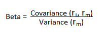
Asset betas typically exhibit time dependency and there are numerous methods that can be used to model this feature, including, for instance, the Kalman Filter:
http://jonathankinlay.com/2015/02/statistical-arbitrage-using-kalman-filter/
Beta Convexity
In the context discussed here we set such matters to one side. Instead of considering how an asset beta may vary over time, we look into how it might change depending on the direction of the benchmark index. To take an example, let’s consider the stock Advaxis, Inc. (Nasdaq: ADXS). In the charts below we examine the relationship between the daily stock returns and the returns in the benchmark Russell 3000 Index when the latter are positive and negative.
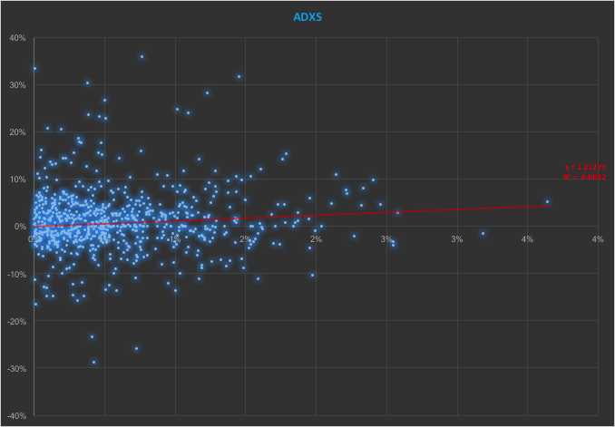
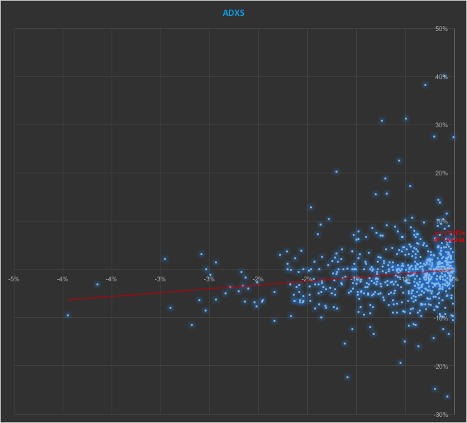
The charts indicate that the stock beta tends to be higher during down periods in the benchmark index than during periods when the benchmark return is positive. This can happen for two reasons: either the correlation between the asset and the index rises, or the volatility of the asset increases, (or perhaps both) when the overall market declines. In fact, over the period from Jan 2012 to May 2017, the overall stock beta was 1.31, but the up-beta was only 0.44 while the down-beta was 1.53. This is quite a marked difference and regardless of whether the change in beta arises from a change in the correlation or in the stock volatility, it could have a significant impact on the optimal weighting for this stock in an equity portfolio.
Ideally, what we would prefer to see is very little dependence in the relationship between the asset beta and the sign of the underlying benchmark. One way to quantify such dependency is with what I have called Beta Convexity:
Beta Convexity = (Up-Beta – Down-Beta) ^2
A stock with a stable beta, i.e. one for which the difference between the up-beta and down-beta is negligibly small, will have a beta-convexity of zero. One the other hand, a stock that shows instability in its beta relationship with the benchmark will tend to have relatively large beta convexity.
Index Replication using a Minimum Beta-Convexity Portfolio
One way to apply this concept it to use it as a means of stock selection. Regardless of whether a stock’s overall beta is large or small, ideally we want its dependency to be as close to zero as possible, i.e. with near-zero beta-convexity. This is likely to produce greater stability in the composition of the optimal portfolio and eliminate unnecessary and undesirable excess volatility in portfolio returns by reducing nonlinearities in the relationship between the portfolio and benchmark returns.
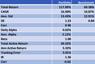
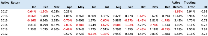
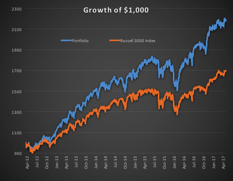
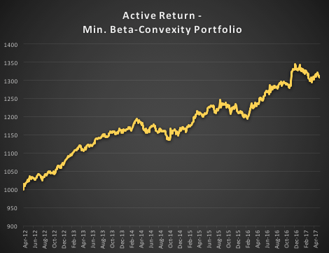
In the following illustration we construct a stock portfolio by choosing the 500 constituents of the benchmark Russell 3000 index that have the lowest beta convexity during the previous 90-day period, rebalancing every quarter (hence all of the results are out-of-sample). The minimum beta-convexity portfolio outperforms the benchmark by a total of 48.6% over the period from Jan 2012-May 2017, with an annual active return of 5.32% and Information Ratio of 1.36. The portfolio tracking error is perhaps rather too large at 3.91%, but perhaps can be further reduced with the inclusion of additional stocks.
Conclusion: Beta Convexity as a New Factor
Beta convexity is a new concept that appears to have a useful role to play in identifying stocks that have stable long term dependency on the benchmark index and constructing index tracking portfolios capable of generating appreciable active returns.
The outperformance of the minimum-convexity portfolio is not the result of a momentum effect, or a systematic bias in the selection of high or low beta stocks. The selection of the 500 lowest beta-convexity stocks in each period is somewhat arbitrary, but illustrates that the approach can scale to a size sufficient to deploy hundreds of millions of dollars of investment capital, or more. A more sensible scheme might be, for example, to select a variable number of stocks based on a predefined tolerance limit on beta-convexity.
Obvious steps from here include experimenting with alternative weighting schemes such as value or beta convexity weighting and further refining the stock selection procedure to reduce the portfolio tracking error.
Further useful applications of the concept are likely to be found in the design of equity long/short and market neural strategies. These I shall leave the reader to explore for now, but I will perhaps return to the topic in a future post.
Strategy Portfolio Construction

Applications of Graph Theory In Finance

Analyzing Big Data
Very large datasets – comprising voluminous numbers of symbols – present challenges for the analyst, not least of which is the difficulty of visualizing relationships between the individual component assets. Absent the visual clues that are often highlighted by graphical images, it is easy for the analyst to overlook important changes in relationships. One means of tackling the problem is with the use of graph theory.
DOW 30 Index Member Stocks Correlation Graph
In this example I have selected a universe of the Dow 30 stocks, together with a sample of commodities and bonds and compiled a database of daily returns over the period from Jan 2012 to Dec 2013. If we want to look at how the assets are correlated, one way is to created an adjacency graph that maps the interrelations between assets that are correlated at some specified level (0.5 of higher, in this illustration).
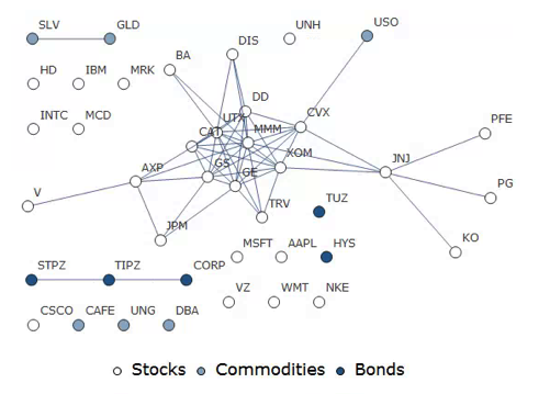
Obviously the choice of correlation threshold is somewhat arbitrary, and it is easy to evaluate the results dynamically, across a wide range of different threshold parameters, say in the range from 0.3 to 0.75:

The choice of parameter (and time frame) may be dependent on the purpose of the analysis: to construct a portfolio we might select a lower threshold value; but if the purpose is to identify pairs for possible statistical arbitrage strategies, one will typically be looking for much higher levels of correlation.
Correlated Cliques
Reverting to the original graph, there is a core group of highly inter-correlated stocks that we can easily identify more clearly using the Mathematica function FindClique to specify graph nodes that have multiple connections:
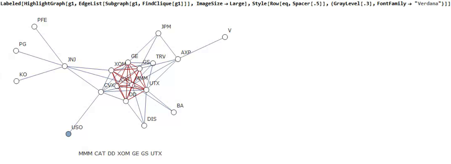
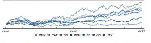
We might, for example, explore the relative performance of members of this sub-group over time and perhaps investigate the question as to whether relative out-performance or under-performance is likely to persist, or, given the correlation characteristics of this group, reverse over time to give a mean-reversion effect.
Constructing a Replicating Portfolio
An obvious application might be to construct a replicating portfolio comprising this equally-weighted sub-group of stocks, and explore how well it tracks the Dow index over time (here I am using the DIA ETF as a proxy for the index, for the sake of convenience):
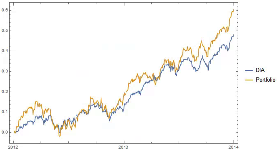
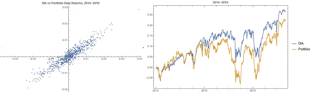
The correlation between the Dow index (DIA ETF) and the portfolio remains strong (around 0.91) throughout the out-of-sample period from 2014-2016, although the performance of the portfolio is distinctly weaker than that of the index ETF after the early part of 2014:
Constructing Robust Portfolios
Another application might be to construct robust portfolios of lower-correlated assets. Here for example we use the graph to identify independent vertices that have very few correlated relationships (designated using the star symbol in the graph below). We can then create an equally weighted portfolio comprising the assets with the lowest correlations and compare its performance against that of the Dow Index.
The new portfolio underperforms the index during 2014, but with lower volatility and average drawdown.

Conclusion – Graph Theory has Applications in Portfolio Constructions and Index Replication
Graph theory clearly has a great many potential applications in finance. It is especially useful as a means of providing a graphical summary of data sets involving a large number of complex interrelationships, which is at the heart of portfolio theory and index replication. Another useful application would be to identify and evaluate correlation and cointegration relationships between pairs or small portfolios of stocks, as they evolve over time, in the context of statistical arbitrage.
Beating the S&P500 Index with a Low Convexity Portfolio
What is Beta Convexity?
Beta convexity is a measure of how stable a stock beta is across market regimes. The essential idea is to evaluate the beta of a stock during down-markets, separately from periods when the market is performing well. By choosing a portfolio of stocks with low beta-convexity we seek to stabilize the overall risk characteristics of our investment portfolio.
A primer on beta convexity and its applications is given in the following post:

In this post I am going to use the beta-convexity concept to construct a long-only equity portfolio capable of out-performing the benchmark S&P 500 index.
The post is in two parts. In the first section I outline the procedure in Mathematica for downloading data and creating a matrix of stock returns for the S&P 500 membership. This is purely about the mechanics, likely to be of interest chiefly to Mathematica users. The code deals with the issues of how to handle stocks with multiple different start dates and missing data, a problem that the analyst is faced with on a regular basis. Details are given in the pdf below. Let’s skip forward to the analysis.
Portfolio Formation & Rebalancing
We begin by importing the data saved using the data retrieval program, which comprises a matrix of (continuously compounded) monthly returns for the S&P500 Index and its constituent stocks. We select a portfolio size of 50 stocks, a test period of 20 years, with a formation period of 60 months and monthly rebalancing.
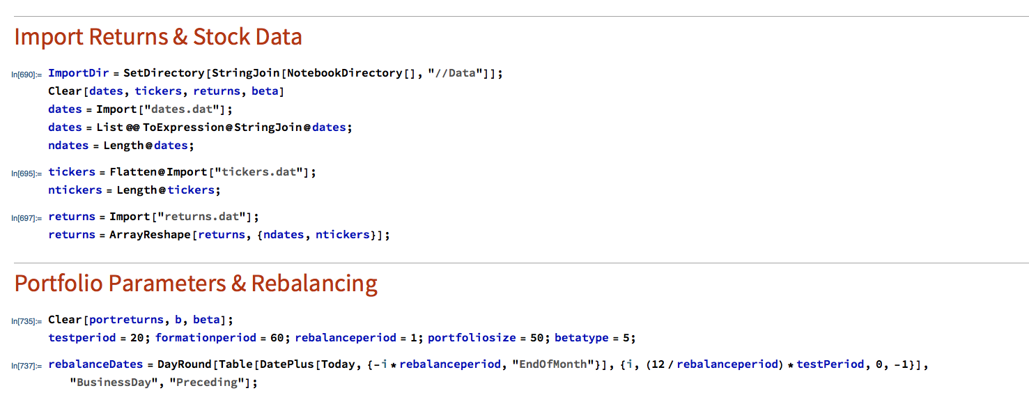
In the processing stage, for each month in our 20-year test period we calculate the beta convexity for each index constituent stock and select the 50 stocks that have the lowest beta-convexity during the prior 5-year formation period. We then compute the returns for an equally weighted basket of the chosen stocks over the following month. After that, we roll forward one month and repeat the exercise.
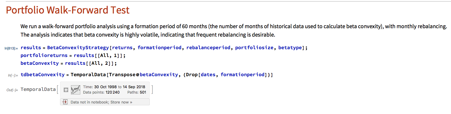
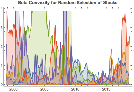
It turns out that beta-convexity tends to be quite unstable, as illustrated for a small sample of component stocks in the chart below:
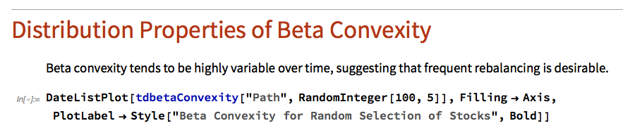
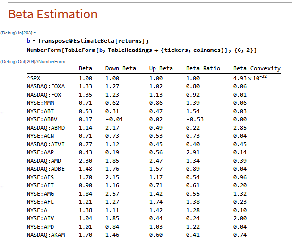
A snapshot of estimated convexity factors is shown in the following table. As you can see, there is considerable cross-sectional dispersion in convexity, in addition to time-series dependency.
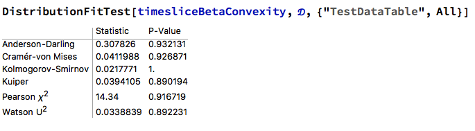
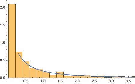
At any point in time the cross-sectional dispersion is well described by a Weibull distribution, which passes all of the usual goodness-of-fit tests.
Performance Results
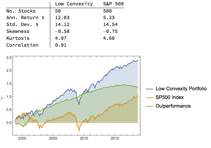
We compare the annual returns and standard deviation of the low convexity portfolio with the S&P500 benchmark in the table below. The results indicate that the average gross annual return of a low-convexity portfolio of 50 stocks is more than double that of the benchmark, with a comparable level of volatility. The portfolio also has slightly higher skewness and kurtosis than the benchmark, both desirable characteristics.
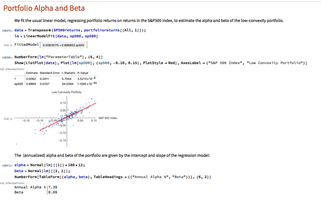
Portfolio Alpha & Beta Estimation
Using the standard linear CAPM model we estimate the annual alpha of the low-convexity portfolio to be around 7.39%, with a beta of 0.89.
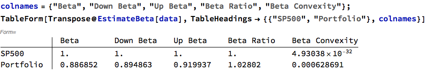
Beta Convexity of the Low Convexity Portfolio
As we might anticipate, the beta convexity of the portfolio is very low since it comprises stocks with the lowest beta-convexity:
Conclusion: Beating the Benchmark S&P500 Index
Using a beta-convexity factor model, we are able to construct a small portfolio that matches the benchmark index in terms of volatility, but with markedly superior annual returns. Larger portfolios offering greater liquidity produce slightly lower alpha, but a 100-200 stock portfolio typically produce at least double the annual rate of return of the benchmark over the 20-year test period.
For those interested, we shall shortly be offering a low-convexity strategy on our Systematic Algotrading platform – see details below:
Section on Data Retrieval and Processing