Why Technical Analysis Doesn’t Work

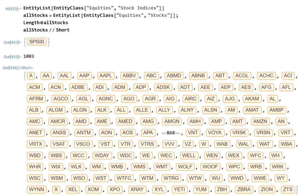
Single Stock Analytics

Generally speaking, one of the major attractions of working in the equities space is that the large number of available securities opens up a much wider range of opportunities for the quantitative researcher than for, say, futures markets.  The focus in equities tends to be on portfolio strategies since the scope of the universe permits an unparalleled degree of diversification.  Single stock strategies forego such benefit, but they are of interest to the analyst and investor nonetheless: “stock picking” is almost a national pastime, at least for US investors.

Rather than seeking to mitigate stock specific risk through diversification,  the stock picker is actively seeking to identify  risk opportunities that are unique  to a specific stock, and he hopes will yield abnormal returns.  These can arise for any number of reasons – mergers and acquisitions, new product development, change in index membership, to name just a few.  The hope is that such opportunities may be uncovered by one of several possible means:

  • Identification of latent, intrinsic value in neglected stocks that has been overlooked by other analysts
  • The use of alternative types of data that permits new insight in the potential of a specific stock or group of stocks
  • A novel method of analysis that reveals hitherto hidden potential in a particular stock or group of stocks

One can think of examples of each of these possibilities, but at the same time it has to be admitted that the challenge is very considerable.  Firstly, your discovery or methodology would have to be one that has eluded some of the brightest minds in the investment industry.  That has happened in the past and will no doubt occur again in future;  but the analyst has to have a fairly high regard for his own intellect – or good fortune – to believe that the golden apple will fall into his lap, rather than another’s. Secondly there is the question of the efficient market hypothesis.  These days it is fashionable to pour scorn  on the EMH, with examples of well-known anomalies often used to justify the opprobrium. But the EMH doesn’t say that markets are 100% efficient, 100% of the time.  It says that markets are efficient, on average.  This  means that there will be times or circumstances in which the market will be efficient and other times and circumstances when it will be relatively inefficient – but you won’t be able to discern which condition the market is in currently.  Finally, even if one is successful in identifying such an opportunity, the benefit has to be realizable and economically significant.  I can think of several examples of equity strategies that appear to offer the potential to generate  alpha, but which turn out to be either unrealizable or economically insignificant after applying transaction costs.

All this is to say that stock picking is one of the most difficult challenges the analyst can undertake.  It is also one of the most interesting challenges – and best paid occupations – on Wall Street.  So it is unsurprising that for analysts it remains the focus of their research and ambition.  In this chapter we will look at some of the ways in which the Equities Entity Store can be used for such purposes and some of the more interesting analytical methods.

Why Technical Analysis Doesn’t Work

Technical Analysis is a very popular approach to analysing stocks.  Unfortunately, it is also largely useless, at least if the intention is to uncover potential sources of alpha.  The reason is not hard to understand: it relies on applying  analytical methods that have been known for decades to widely available public information (price data).  There  isn’t any source of competitive advantage that might reliably produce abnormal returns.  Even the possibility  of uncovering a gem amongst the stocks overlooked by other analysts appears increasingly remote these days, as the advent of computerized trading systems has facilitated the application of standard technical analysis tools on an industrial scale.  You don’t even need to understand how the indicators work – much less how to program them – in order to apply them to tens of thousands of stocks.  

And yet Technical Analysis remains very popular.  Why so?  The answer, I believe, is because it’s easy to do and can often look very pretty.  I will go further and admit that some of the indicators that analysts have devised are extraordinarily creative.  But they just don’t work.  In fact, I can’t think of another field of human industry that engages so many inventive minds in such a fruitless endeavor.  

All this has been clear for some time and yet every year legions of newly minted analysts fling themselves into the task of learning how to apply Technical Analysis to everything from cattle futures to cryptocurrencies.  Realistically, the chances of my making any kind of impression on this torrent of pointless hyperactivity are close to zero, but I will give it a go.
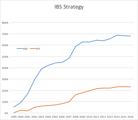
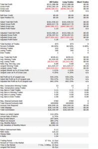
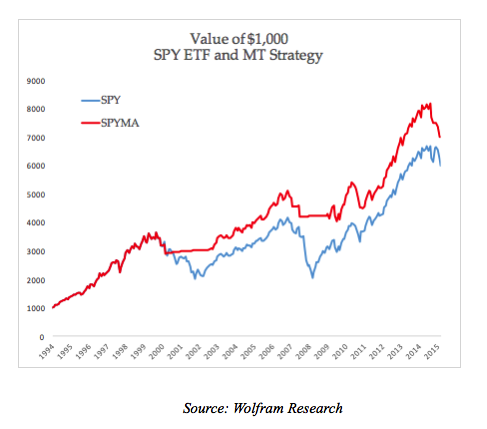
A Demonstration

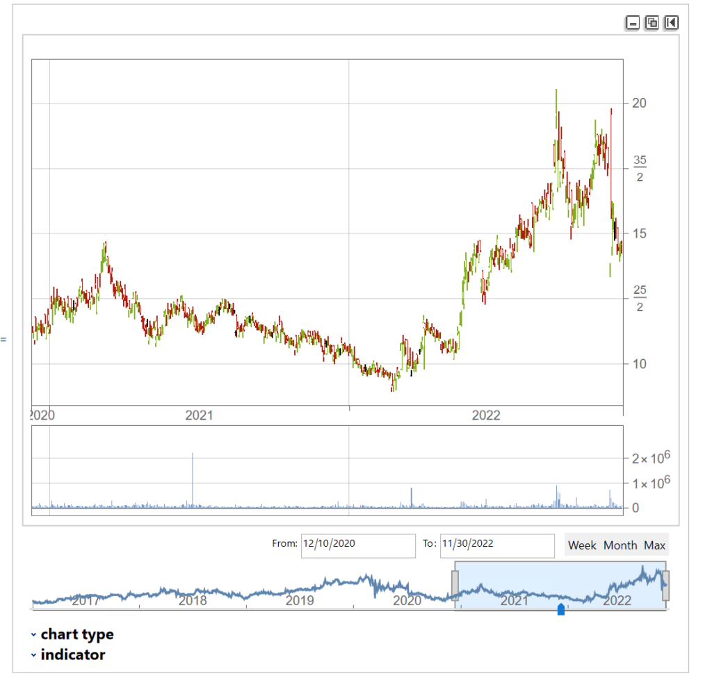
Let’ s begin by picking a stock at random, one I haven’ t look at previously :

waterUtilities=Select[allListedStocks,#["Sector Information"]["GICS Industry"]== "Water Utilities"&]

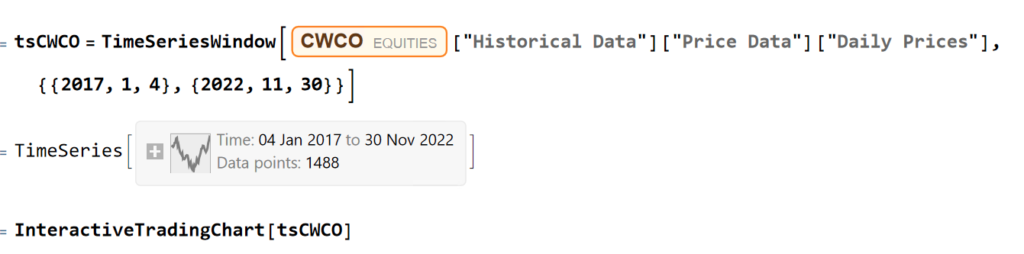
We’ll extract a daily price series from 2017 to 2022 and plot an interactive trading chart, to which we can add moving averages, or any number of other technical indicators, as we wish:

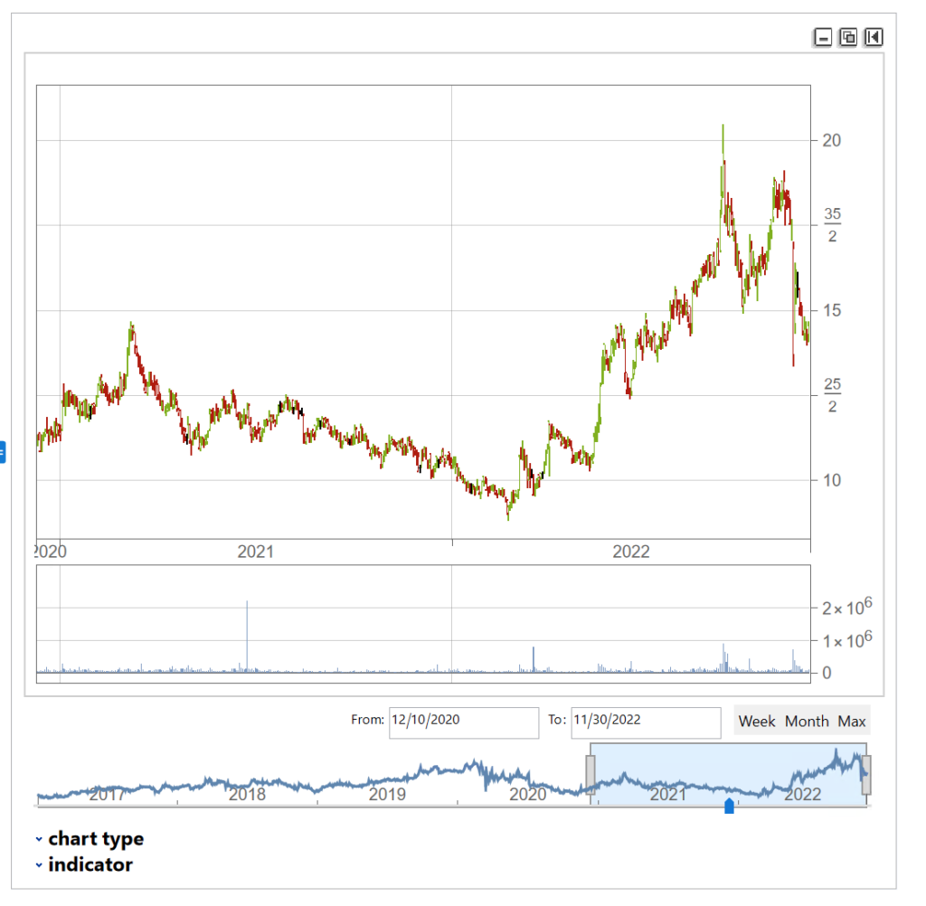
The chart shows several different types of pattern that are well-known to technical analysis, including trends, continuation patterns, gaps, double tops, etc

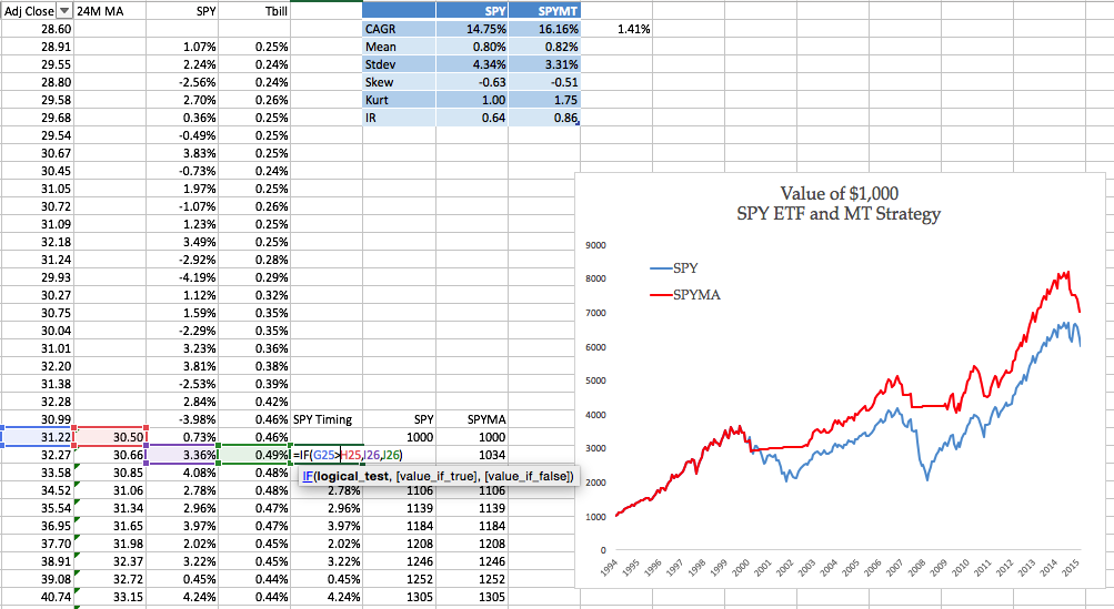
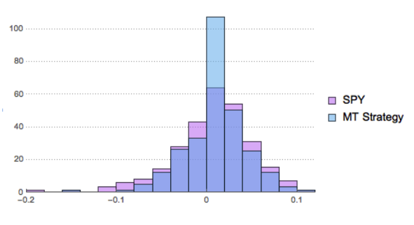
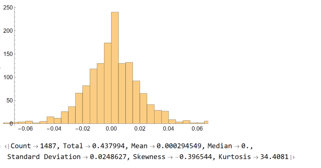
Let’ s look at the pattern of daily returns:

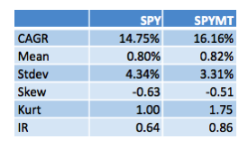
returns=Differences@Log[tsCWCO["PathComponent",4]["Values"]];
Histogram[returns]
stats=ReturnStatistics[returns]

Next, we will generate a series of random returns, drawn from a Gaussian distribution with the same mean and standard deviation as the empirical returns series:

randomreturns=RandomVariate[NormalDistribution[stats["Mean"],stats["Standard Deviation"]],Length[returns]];
Histogram[randomreturns]
ReturnStatistics[randomreturns]

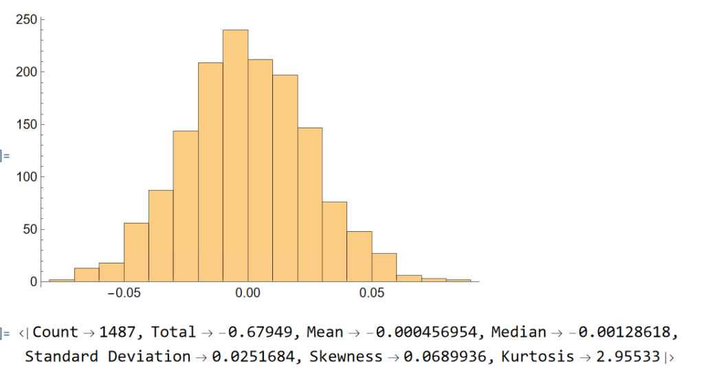
Clearly, the distribution of the generated returns differs from the distribution of empirical returns, but that doesn’t matter:  all that counts is that we can agree that the generated returns, which represent the changes in (log) prices from one day to the next, are completely random. Consequently, knowing the random returns, or prices,  at time t  = 1, 2, . . . , (t-1) in no way enables you to forecast the return , or price, at time t.

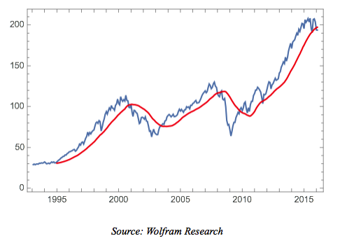
Now let’ s generate a series of synthetic prices  and time series, using the synthetic returns to calculate the prices for each period:

syntheticPrices=Exp[FoldList[Plus,Log[First[tsCWCO["FirstValues"]][[1;;4]]],Transpose[ConstantArray[returns,4]]]];

tsSynthetic=TimeSeries[ArrayFlatten@{{syntheticPrices,List/@tsCWCO["PathComponent",5]["Values"]}},{tsCWCO["Dates"]}]

InteractiveTradingChart[tsSynthetic]

The synthetic time series is very similar to the original and displays many of the same characteristics, including classical patterns that are immediately comprehensible to a technical analyst, such as gaps, reversals , double tops, etc.

But the two time series, although similar,  are not identical:

tsCWCO===tsSynthetic

False

We knew this already, of course, because we used randomly generated returns to create the synthetic price series.  What this means is that, unlike for the real price series, in the case of the synthetic price series we know for certain that the movement in prices from one period to the next is entirely random.  So if prices continue in an upward trend after a gap, or decline after a double top formation appears on the chart of the synthetic series, that happens entirely by random chance, not in response to a pattern flagged by the technical indicator.  If we had generated a different set of random returns, we could just as easily have produced a synthetic price series in which prices reversed after a gap up, or continued higher after a double-top formation.  Critics of Technical Analysis do not claim that patterns such as gaps, head and shoulders , etc., do not exist – they clearly do.  Rather, we say that such patterns are naturally occurring phenomena that will arise even in a series known to be completely random and hence can have no economic significance.

The point is not to say that technical signals never work: sometimes they do and sometimes they don’t.  Rather, the point is that, in any given situation, you will be unable to tell whether the signal is going to work this time, or not – because price changes are  dominated by random variation.  

You can make money in the markets using technical analysis, just as you can by picking stocks at random, throwing darts at a dartboard, or tossing a coin to decide which to buy or sell – i.e. by dumb luck.  But you can’t reliably make money this way.

  • More on the efficient market hypothesis
  • More from the Society of Technical Analysts

Equity Analytics in the Equities Data Store

Equities Entity Store  – A Brief Review

The Equities Entity Store applies the object-oriented concept of Entity Stores in the Wolfram Language to create a collection of equity objects, both stocks and stock indices, containing current and historical fundamental, technical and performance-related data. Also included in the release version of the product will be a collection of utility functions (a.k.a. “Methods”) that will facilitate equity analysis,  the formation and evaluation of equity portfolios and the development and back-testing of equities strategies, including cross-sectional strategies.

In the pre-release version of the store there are just over 1,000 equities, but this will rise to over 2,000 in the first release, as delisted securities are added to the store. This is important in order to eliminate survivor bias from the data set.

First Release of the Equities Entity Store – January 2023

The first release of the equities entity store product will contain around 2,000-2,500 equities, including at least 1,000 active stocks listed on the NYSE and NASDAQ exchanges and a further 1,000-1,500 delisted securities. All of the above information will be available for each equity and, in addition, the historical data will include quarterly fundamental data.

The other major component of the store will be analytics tools, including single-stock analytics functions such as those illustrated here. More important, however, is that the store will contain advanced analytics tools designed to assist the analyst in the construction of optimized equity portfolios and in the development and backtesting of long and long/short equity strategies.

Readers wishing to receive more information should contact me at algosciences (at) gmail.com

The Internal Bar Strength Indicator

Internal Bar Strength (IBS) is an idea that has been around for some time.  IBS is based on the position of the day’s close in relation to the day’s range: it takes a value of 0 if the closing price is the lowest price of the day, and 1 if the closing price is the highest price of the day.

More formally:

IBS  =  (Close – Low) / (High – Low)

The IBS effect may be related to intraday over-reaction to news or market movements, which are then ”corrected” the next day.  It serves as a measure of the tendency of a price series to mean-revert over daily horizons.  I use the term “daily” advisedly: so far as I am aware, there has been no research (including my own) demonstrating the existence of an IBS effect at time horizons shorter, or longer, than one day.  Indeed, there has been very little in the way of academic research into the concept of any kind, which is strange considering how compelling are the results it is capable of producing.  Practitioners have been happy enough with that state of affairs, content to deploy this neglected indicator in their trading strategies, where it has often proved to be extremely useful (we use IBS in one of our volatility strategies). Since 2013, however, the cat has been let out of the bag, thanks to an excellent research paper by Alexander Pagonidis, who writes an interesting quantitative finance blog.

The essence of the idea is that stocks that close in the lowest part of the daily range, with an IBS of below, say, 0.2, will tend to rally the next day, while stocks that close in the highest quintile will often decline in value in the following session.  In his paper “The IBS Effect: Mean Reversion in Equity ETFs” (2013), Pagonidis researches the IBS effect in equity index ETFs in the US and several international markets.  He confirms that low IBS values in these assets are associated with high returns in the following day session, while high IBS values are associated with low returns. Average returns when IBS is below 0.20 are .35% ,while average returns when IBS is above 0.80 are -0.13%. According to his research, this effect has been present in equity ETFs since the early 90s and has been highly consistent through time.

SSALGOTRADING AD

IBS Strategy Performance

To give the reader some idea of the potential of the IBS effect, I have reproduced below equity curves for the IBS strategy for the SPDR S&P 500 ETF Trust (SPY) and iShares MSCI Singapore ETF (EWS) index ETFs over the period from 1999 to 2016.  The strategy buys at the close when IBS is below 0.2, and sells at the close when IBS exceeds 0.8, liquidating the position at the following market close. Strategy CAGR over the period has been of the order of 13% for SPY and as high as 40% for EWS, ignoring transaction costs.

IBS Strategy Chart SPY EWS


Note that in both cases strategy returns for SPY and EWS have diminished in recent years, turning negative in 2015 and 2016 YTD and this is true for ETFs in general.  It remains to be seen whether this deterioration in strategy performance is temporary or permanent.  There are some indications that the latter holds true, but the evidence is not quite definitive.  For example, the chart below shows daily equity curve for the SPY IBS strategy, with 95% confidence intervals for the latest 100 trades (up to the end of May 2016), constructed using Monte-Carlo bootstrap.  The equity curve appears to have penetrated the lower bound, indicating a statistically significant deterioration in the performance of the IBS strategy for SPY over the last year or so (EWS is similar).  That said, the equity curve does fall inside the boundaries of the 99% confidence interval, so those looking for greater certainty about the possible breakdown of the effect will need to wait a little longer for confirmation.


SPY IBS MSA


Whatever the outcome may be for SPY and other ETFs going forward, it is certainly true that IBS effects persist strongly for some individual equities, Exxon-Mobil Corp. (XOM) being a case in point (see below).  It’s worth taking note of the exceptional performance of the XOM IBS strategy during the latter quarter of 2008.  I will have much more to say on the application of the IBS indicator for individual equities in a future blog post.


XOM IBS Strategy


The Role of Range, Volume, Bull/Bear Markets, Volatility and Seasonality

Pagonidis goes on to detail several further important findings in relation to IBS.  It is clear from his research that high volatility is related to increased predictability of returns and a more powerful IBS effect, in particular the high IBS-negative return aspect.  As might be expected, the effect is also larger after days with high range, both for high and low IBS extremes.

Volume turns out to be especially important for  U.S. index ETFs:  in fact, the IBS effect only appears to work on high-volume days.

Pagonidis also separates the data into bull and bear market environments, based on whether 200-day returns are positive or not.  The size of the effect is roughly similar in each environment (slightly larger in bear markets), but it is greater in the direction of the overall trend: high IBS readings are followed by larger negative returns during bear markets, and vice versa.

Day of Week Effect

The IBS effect is also strongly seasonal, having the greatest impact on returns from Monday’s close to Tuesday’s close, as illustrated for the SPY ETF in the chart below.  This accounts for the phenomenon known popularly as “Turnaround Tuesday”, i.e. the tendency for the market to recover strongly from losses on a Monday.  The day-of-week effect is weakest for Fridays.


SPY DOW


The mean of the returns distribution is not the only aspect that IBS can predict. Skewness also varies significantly between IBS buckets, with low IBS readings being followed by highly skewed returns, and vice versa. Close-to-close returns after a bottom-bucket IBS day have average skewness of 0.65 across Equity Index ETF products, while top-bucket IBS days are followed by returns with skewness of 0.03. This finding has very useful risk management applications for investors concerned with tail risk.

IBS as a Filter for a Swing Trading Strategy in QQQ

The returns to an IBS-only strategy are both statistically and economically significant. However, commissions will greatly decrease the returns and increase the maximum drawdowns, however, making such an approach challenging in the real world. One alternative is to combine the IBS effect with mean reversion on longer timescales and only take trades when they align.

Pagonidis offers a simple demonstration using the Cutler’s RSI indicator that shows how the IBS effect can be used to boost returns of a swing trading strategy while significantly decreasing the number of trades needed.

Cutler’s RSI at time t is calculated as follows:


RSI


Pagonidis tests a simple, long-only strategy that trades the PowerShares QQQ Trust, Series 1 (QQQ) ETF using the Cutler’s RSI(3) indicator:

• Go long at the close if RSI(3) < 10

• Maintain the position while RSI(3) ≤ 40

 filter these returns by adding an additional rule based on the value of IBS:

• Enter or maintain long position only if IBS ≤ 0.5

Pangonis claims that the strategy produces rather promising results that “easily beats commissions”;  however, my own rendition of the strategy, assuming commissions of $0.005 per share and slippage of a further $0.02 per share produces results that are distinctly less encouraging:

EC0


Pef0

Strategy Code

For those interested, the code is as follows:

Inputs:
RSILen(3),
RSI_Entry(10),
RSI_Exit(40),
IBS_Threshold(0.5),
Initial_Capital(100000);
Vars:
nShares(100),
RSIval(0),
IBS(0);
RSIval=RSI(C,RSILen);
IBS = (C-L)/(H-L);

nShares = Round(Initial_Capital / Close,0);

If Marketposition = 0 and RSIval > RSI_Entry and IBS < IBS_Threshold then begin
Buy nShares contracts next bar at market;
end;
If Marketposition > 0 and ((RSIval > RSI_Exit) or (IBS_Threshold > IBS_Threshold)) then begin
Sell next bar at market;
end;

Strategy Optimization and Robustness Testing

One can further improve performance by optimizing the trading system parameters, using Tradestation’s excellent Walk Forward Optimization (WFO) module.  This allows us to examine the effect of re-calibrating the strategy parameters are regular intervals, testing the optimized model on out-of-sample data sets of various sizes.  WFO can be used, not only optimize a strategy, but also to examine the sensitivity of its performance to changes in the levels of key parameters.  For example, in the case of the QQQ swing trading strategy, we find that profitability increases monotonically with the length of the RSI indicator, and this effect is especially marked when an IBS threshold level of 0.2 is used:

Sensitivity


Likewise we can test the consistency of the day-of-the-week effect over several OS data sets of  varying size and these tests are consistent with the pattern seen earlier for the IBS indicator, confirming its role as a filter rule in enhancing system profitability:

Distribution Analysis


A model that is regularly re-calibrated using WFO is subjected to a series of tests designed to ensure its robustness and consistency in live trading.   The tests include the following:


WFO


In order to achieve an overall pass rating, the system is required to pass all five tests of its out-of-sample performance, from which Tradestation deems it likely that the system will continue to perform well in live trading.  The results from this procedure appear much more promising than the strategy in its original form, as can be seen from the performance table and equity curve chart shown below.

EC1

Perf1


However, these results include both in-sample and out-of-sample periods.  An examination of the results from the WFO indicate that the overall efficiency of the strategy is around 55%, meaning that the P&L produced by the system in out-of-sample periods amounts to a little over one half of the rate of profit produced during in-sample periods.  Going forward, therefore, we might expect the performance of the system in live trading to be only around half as good as shown here.  While this is still superior to the original system, it may not be considered good enough.  Nonetheless, for the purpose of illustrating the benefits of the IBS indicator as a trade filter, it makes the point.

Another interesting example of an IBS-based trading strategy in the QQQ and SPY ETFs can be found in the following blog post.

Conclusion

Internal Bar Strength is a powerful mean-reversion indicator for equity products traded at daily frequencies, with a consistent effect that has continued from the 1990s through to the current decade. IBS can be used on its own in mean-reversion strategies that have worked well for both US equities and US and International equity index ETFs, or used as a trade filter when combined with other alpha signals.

While there is evidence of a weakening of the IBS effect since around 2013 this is not yet confirmed statistically (at the 99% confidence level) and may simply be the result of normal statistical variation in its efficacy.


Some Further Notes on Market Timing

Almost at the very moment I published a post featuring some interesting research by Glabadanidis (“Market Timing With Moving Averages”  (2015), International Review of Finance, Volume 15, Number 13, Pages 387-425 – see Yes, You Can Time the Market. How it Works, And Why), several readers wrote to point out a recently published paper by Valeriy Zakamulin, (dubbed the “Moving Average Research King” by Alpha Architect, the source for our fetching cover shot) debunking Glabadanidis’s findings in no uncertain terms:

We demonstrate that “too good to be true” reported performance of the moving average strategy is due to simulating the trading with look-ahead bias. We perform the simulations without look-ahead bias and report the true performance of the moving average strategy. We find that at best the performance of the moving average strategy is only marginally better than that of the corresponding buy-and-hold strategy.

So far, no response from Glabadanidis – from which one is tempted to conclude that Zakamulin is correct.

I can’t recall the last time a paper published in a leading academic journal turned out to be so fundamentally flawed.  That’s why papers are supposed to be peer reviewed.   But, I guess, it can happen. Still, it’s rather alarming to think that a respected journal could accept a piece of research as shoddy as Zakamulin claims it to be.

What Glabadanidis had done, according to Zakamulin, was to use the current month closing price to compute the moving average that was used to decide whether to exit the market (or remain invested) at the start of the same month.  An elementary error that introduces look-ahead bias that profoundly impacts the results.

Following this revelation I hastily checked my calculations for the SPY marketing timing  strategy illustrated in my blog post and, to my relief, confirmed that I had avoided the look-ahead trap that Glabadanidis has fallen into.  As the reader can see from the following extract from the Excel spreadsheet I used for the calculations, the decision to assume the returns for the SPY ETF or T-Bills for the current month rests on the value of the 24 month MA computed using prices up to the end of the prior month.  In other words, my own findings are sound, even if Glabadanidis’s are not, as the reader can easily check for himself.


Excel Workbook


Nonetheless, despite my relief at having avoided Glabadanidis’s  blunder, the apparent refutation of his findings comes as a disappointment.  And my own research on the SPY market timing strategy, while sound as far as it goes, cannot by itself rehabilitate the concept of market timing using moving averages.  The reason is given in the earlier post.  There is a hidden penalty involved in using the market timing strategy to synthetically replicate an Asian put option, namely the costs incurred in exiting and rebuilding the portfolio as the market declines below the moving average, or later overtakes it.  In a single instance, such as the case of SPY, it might easily transpire simply by random chance that the cost of replication are far lower than the fair value of the put.  But the whole point of Glabadanidis’s research was that the same was true, not only for a single ETF or stock, but for many thousands of them.  Absent that critical finding, the SPY case is no more than an interesting anomaly.

Finally, one reader pointed out that the effect of combining a put option with a stock (or ETF) long position was to create synthetically a call option in the stock (ETF).  He is quite correct.  The key point, however, is that when the stock trades down below its moving average, the value of the long synthetic call position and the market timing portfolio are equivalent.


Yes, You Can Time the Market. How it Works, And Why

One of the most commonly cited maxims is that market timing is impossible.  In fact, empirical evidence makes a compelling case that market timing is feasible and can yield substantial economic benefits.  What’s more, we even understand why it works.  For the typical portfolio investor, applying simple techniques to adjust their market exposure can prevent substantial losses during market downturns.

The Background From Empirical and Theoretical Research

For the last fifty years, since the work of Paul Samuelson, the prevailing view amongst economists has been that markets are (mostly) efficient and follow a random walk. Empirical evidence to the contrary was mostly regarded as anomalous and/or unimportant economically.  Over time, however, evidence has accumulated that market effects may persist that are exploitable. The famous 1992 paper published by Fama and French, for example, identified important economic effects in stock returns due to size and value factors, while Cahart (1997) demonstrated the important incremental effect of momentum.  The combined four-factor Cahart model explains around 50% of the variation in stock returns, but leaves a large proportion that cannot be accounted for.

Other empirical studies have provided evidence that stock returns are predictable at various frequencies.  Important examples include work by Brock, Lakonishok and LeBaron (1992), Pesaran and Timmermann (1995) and Lo, Mamaysky and Wang (2000), who provide further evidence using a range of technical indicators with wide popularity among traders showing that this adds value even at the individual stock level over and above the performance of a stock index.  The research in these and other papers tends to be exceptional in term of both quality and comprehensiveness, as one might expect from academics risking their reputations in taking on established theory.  The appendix of test results to the Pesaran and Timmermann study, for example, is so lengthy that is available only in CD-ROM format.

A more recent example is the work of Paskalis Glabadanidis, in a 2012 paper entitled Market Timing with Moving Averages.  Glabadanidis examines a simple moving average strategy that, he finds, produces economically and statistically significant alphas of 10% to 15% per year, after transaction costs, and which are largely insensitive to the four Cahart factors. 

Glabadanidis reports evidence regarding the profitability of the MA strategy in seven international stock markets. The performance of the MA strategies also holds for more than 18,000 individual stocks. He finds that:

“The substantial market timing ability of the MA strategy appears to be the main driver of the abnormal returns.”

An Illustration of a Simple Marketing Timing Strategy in SPY

It is impossible to do justice to Glabadanidis’s research in a brief article and the interested reader is recommended to review the paper in full.  However, we can illustrate the essence of the idea using the SPY ETF as an example.   

A 24-period moving average of the monthly price series over the period from 1993 to 2016 is plotted in red in the chart below.

Fig1

The moving average indicator is used to time the market using the following simple rule:

if Pt >= MAt  invest in SPY in month t+1

if Pt < MAt  invest in T-bills in month t+1

In other words, we invest or remain invested in SPY when the monthly closing price of the ETF lies at or above the 24-month moving average, otherwise we switch our investment to T-Bills.

The process of switching our investment will naturally incur transaction costs and these are included in the net monthly returns.

The outcome of the strategy in terms of compound growth is compared to the original long-only SPY investment in the following chart.

Fig2

The marketing timing strategy outperforms the long-only ETF,  with a CAGR of 16.16% vs. 14.75% (net of transaction costs), largely due to its avoidance of the major market sell-offs in 2000-2003 and 2008-2009.

But the improvement isn’t limited to a 141bp improvement in annual compound returns.  The chart below compares the distributions of monthly returns in the SPY ETF and market timing strategy.

Fig3

It is clear that, in addition to a higher average monthly return, the market timing strategy has lower dispersion in the distribution in returns.  This leads to a significantly higher information ratio for the strategy compared to the long-only ETF.  Nor is that all:  the market timing strategy has both higher skewness and kurtosis, both desirable features.

Fig4

These results are entirely consistent with Glabadanidis’s research.  He finds that the performance of the market timing strategy is robust to different lags of the moving average and in subperiods, while investor sentiment, liquidity risks, business cycles, up and down markets, and the default spread cannot fully account for its performance. The strategy works just as well with randomly generated returns and bootstrapped returns as it does for the more than 18,000 stocks in the study.

A follow-up study by the author applying the same methodology to a universe of 20 REIT indices and 274 individual REITs reaches largely similar conclusions.

Why Marketing Timing Works

For many investors, empirical evidence – compelling though it may be – is not enough to make market timing a credible strategy, absent some kind of “fundamental” explanation of why it works.  Unusually, in the case of the simple moving average strategy, such explanation is possible.

It was Cox, Ross and Rubinstein who in 1979 developed the binomial model as a numerical method for pricing options.  The methodology relies on the concept of option replication, in which one constructs a portfolio comprising holdings of the underlying stock and bonds to produce the same cash flows as the option at every point in time (the proportion of stock to hold is given by the option delta).  Since the replicating portfolio produces the same cash flows as the option, it must have the same value and since once knows the price of the stock and bond at each point in time one can therefore price the option.  For those interested in the detail, Wikipedia gives a detailed explanation of the technique.

We can apply the concept of option replication to construct something very close the MA market timing strategy, as follows.  Consider what happens when the ETF falls below the moving average level.  In that case we convert the ETF portfolio to cash and use the proceeds to acquire T-Bills.  An equivalent outcome would be achieved by continuing to hold our long ETF position and acquiring a put option to hedge it.  The combination of a long ETF position, and a 1-month put option with delta of -1, would provide the same riskless payoff as the market timing strategy, i.e. the return on 30-day T-Bills.  An option in which the strike price is based on the average price of the underlying is known as an Arithmetic Asian option.    Hence when we apply the MA timing strategy we are effectively constructing a dynamic portfolio that replicates the payoff of an Arithmetic Asian protective put option struck as (just above) the moving average level.

Market Timing Alpha and The Cost of Hedging

None of this explanation is particularly contentious – the theory behind option replication through dynamic hedging is well understood – and it provides a largely complete understanding of the way the MA market timing strategy works, one that should satisfy those who are otherwise unpersuaded by arguments purely from empirical research.

There is one aspect of the foregoing description that remains a puzzle, however.  An option is a valuable financial instrument and the owner of a protective put of the kind described can expect to pay a price amounting to tens or perhaps hundreds of basis points.  Of course, in the market timing strategy we are not purchasing a put option per se, but creating one synthetically through dynamic replication.  The cost of creating this synthetic equivalent comprises the transaction costs incurred as we liquidate and re-assemble our portfolio from month to month, in the form of bid/ask spread and commissions.  According to efficient market theory, one should be indifferent as to whether one purchases the option at a fair market price or constructs it synthetically through replication – the cost should be equivalent in either case.  And yet in empirical tests the cost of the synthetic protective put falls far short of what one would expect to pay for an equivalent option instrument.  This is, in fact, the source of the alpha in the market timing strategy.

According to efficient market theory one might expect to pay something of the order of 140 basis points a year in transaction costs – the difference between the CAGR of the market timing strategy and the SPY ETF – in order to construct the protective put.  Yet, we find that no such costs are incurred.

Now, it might be argued that there is a hidden cost not revealed in our simple study of a market timing strategy applied to a single underlying ETF, which is the potential costs that could be incurred if the ETF should repeatedly cross and re-cross the level of the moving average, month after month.  In those circumstances the transaction costs would be much higher than indicated here.  The fact that, in a single example, such costs do not arise does not detract in any way from the potential for such a scenario to play out. Therefore, the argument goes, the actual costs from the strategy are likely to prove much higher over time, or when implemented for a large number of stocks.

All well and good, but this is precisely the scenario that Glabadanidis’s research addresses, by examining the outcomes, not only for tens of thousands of stocks, but also using a large number of scenarios generated from random and/or bootstrapped returns.  If the explanation offered did indeed account for the hidden costs of hedging, it would have been evident in the research findings.

Instead, Glabadanidis concludes:

“This switching strategy does not involve any heavy trading when implemented with break-even transaction costs, suggesting that it will be actionable even for small investors.”

Implications For Current Market Conditions

As at the time of writing, in mid-February 2016, the price of the SPY ETF remains just above the 24-month moving average level.  Consequently the market timing strategy implies one should continue to hold the market portfolio for the time being, although that could change very shortly, given recent market action.

Conclusion

The empirical evidence that market timing strategies produce significant alphas is difficult to challenge.  Furthermore, we have reached an understanding of why they work, from an application of widely accepted option replication theory. It appears that using a simple moving average to time market entries and exits is approximately equivalent to hedging a portfolio with a protective Arithmetic Asian put option.

What remains to be answered is why the cost of constructing put protection synthetically is so low.  At the current time, research indicates that market timing strategies consequently are able to generate alphas of 10% to 15% per annum.

References

  1. Brock, W., Lakonishok, J., LeBaron, B., 1992, “Simple Technical Trading Rules and the Stochastic Properties of Stock Returns,” Journal of Finance 47, pp. 1731-1764.
  2. Carhart, M. M., 1997, “On Persistence in Mutual Fund Performance,” Journal of Finance 52, pp. 57–82.

  3. Fama, E. F., French, K. R., 1992, “The Cross-Section of Expected Stock Returns,” Journal of Finance 47(2), 427–465
  4. Glabadanidis, P., 2012, “Market Timing with Moving Averages”, 25th Australasian Finance and Banking Conference.
  5. Glabadanidis, P., 2012, “The Market Timing Power of Moving Averages: Evidence from US REITs and REIT Indexes”, University of Adelaide Business School.
  6. Lo, A., Mamaysky, H., Wang, J., 2000, “Foundations of Technical Analysis: Computational Algorithms, Statistical Inference, and Empirical Implementation,” Journal of Finance 55, 1705–1765.
  7. Pesaran, M.H., Timmermann, A.G., 1995, “Predictability of Stock Returns: Robustness and Economic Significance”, Journal of Finance, Vol. 50 No. 4