Developing Trading Strategies With Synthetic Data

One of the main criticisms levelled at systematic trading over the last few years is that the over-use of historical market data has tended to produce curve-fitted strategies that perform poorly out of sample in a live trading environment. This is indeed a valid criticism – given enough attempts one is bound to arrive eventually at a strategy that performs well in backtest, even on a holdout data sample. But that by no means guarantees that the strategy will continue to perform well going forward.

The solution to the problem has been clear for some time: what is required is a method of producing synthetic market data that can be used to build a strategy and test it under a wide variety of simulated market conditions. A strategy built in this way is more likely to survive the challenge of live trading than one that has been developed using only a single historical data path.

The problem, however, has been in implementation. Up until now all the attempts to produce credible synthetic price data have failed, for one reason or another, as I described in an earlier post:

I have been able to devise a completely new algorithm for generating artificial price series that meet all of the key requirements, as follows:

  • Computational simplicity & efficiency. Important if we are looking to mass-produce synthetic series for a large number of assets, for a variety of different applications. Some deep learning methods would struggle to meet this requirement, even supposing that transfer learning is possible.
  • The ability to produce price series that are internally consistent (i.e High > Low, etc) in every case .
  • Should be able to produce a range of synthetic series that vary widely in their correspondence to the original price series. In some case we want synthetic price series that are highly correlated to the original; in other cases we might want to test our investment portfolio or risk control systems under extreme conditions never before seen in the market.
  • The distribution of returns in the synthetic series should closely match the historical series, being non-Gaussian and with “fat-tails”.
  • The ability to incorporate long memory effects in the sequence of returns.
  • The ability to model GARCH effects in the returns process.

This means that we are now in a position to develop trading strategies without any direct reference to the underlying market data. Consequently we can then use all of the real market data for out-of-sample back-testing.

Developing a Trading Strategy for the S&P 500 Index Using Synthetic Market Data

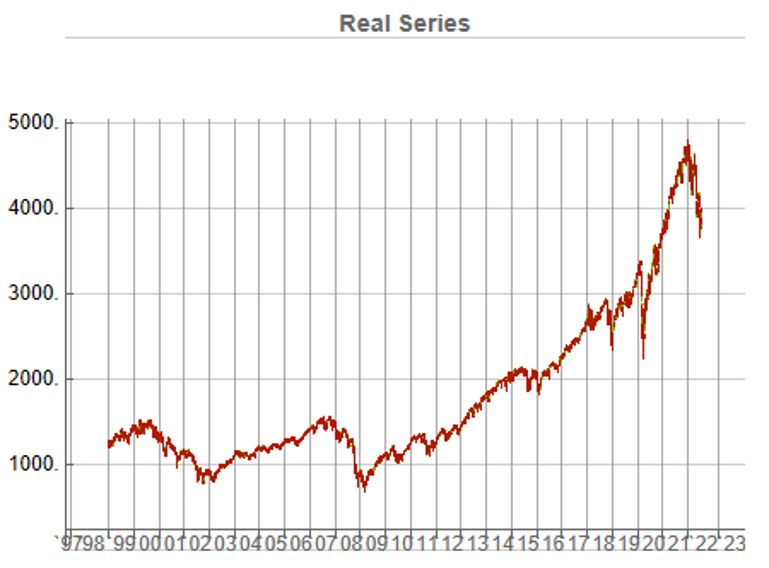
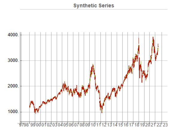
To illustrate the procedure I am going to use daily synthetic price data for the S&P 500 Index over the period from Jan 1999 to July 2022. Details of the the characteristics of the synthetic series are given in the post referred to above.
This image has an empty alt attribute; its file name is Fig3-12.png

Because we want to create a trading strategy that will perform under market conditions close to those currently prevailing, I will downsample the synthetic series to include only those that correlate quite closely, i.e. with a minimum correlation of 0.75, with the real price data.

Why do this? Surely if we want to make a strategy as robust as possible we should use all of the synthetic data series for model development?

The reason is that I believe that some of the more extreme adverse scenarios generated by the algorithm may occur quite rarely, perhaps once in every few decades. However, I am principally interested in a strategy that I can apply under current market conditions and I am prepared to take my chances that the worst-case scenarios are unlikely to come about any time soon. This is a major design decision, one that you may disagree with. Of course, one could make use of every available synthetic data series in the development of the trading model and by doing so it is likely that you would produce a model that is more robust. But the training could take longer and the performance during normal market conditions may not be as good.

Having generated the price series, the process I am going to follow is to use genetic programming to develop trading strategies that will be evaluated on all of the synthetic data series simultaneously. I will then use the performance of the aggregate portfolio, i.e. the outcome of all of the trades generated by the strategy when applied to all of the synthetic series, to assess the overall performance. In order to be considered, candidate strategies have to perform well under all of the different market scenarios, or at least the great majority of them. This ensures that the strategy is likely to prove more robust across different types of market conditions, rather than on just the single type of market scenario observed in the real historical series.

As usual in these cases I will reserve a portion (10%) of each data series for testing each strategy, and a further 10% sample for out-of-sample validation. This isn’t strictly necessary: since the real data series has not be used directly in the development of the trading system, we can later test the strategy on all of the historical data and regard this as an out-of-sample backtest.

To implement the procedure I am going to use Mike Bryant’s excellent Adaptrade Builder software.

This is an exemplar of outstanding software engineering and provides a broad range of features for generating trading strategies of every kind. One feature of Builder that is particularly useful in this context is its ability to construct strategies and test them on up to 20 data series concurrently. This enables us to develop a strategy using all of the synthetic data series simultaneously, showing the performance of each individual strategy as well for as the aggregate portfolio.

After evolving strategies for 50 generations we arrive at the following outcome:
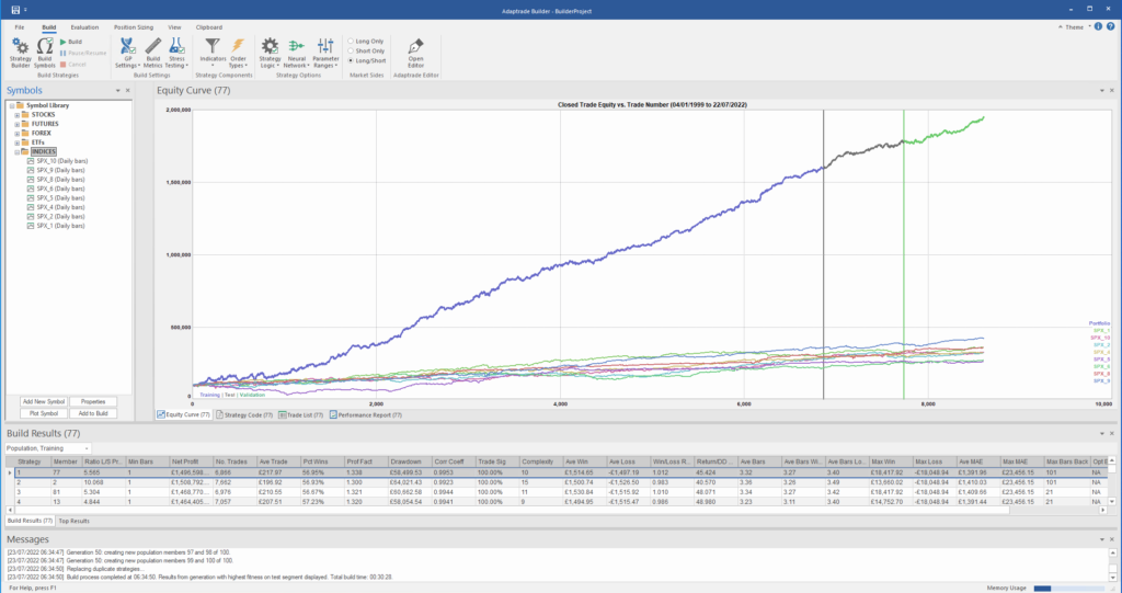
The equity curve for the aggregate portfolio is shown in blue, while the equity curves for the strategy applied to individual synthetic data series are shown towards the bottom of the chart. Of course, the performance of the aggregate portfolio appears much superior to any of the individual strategies, because it is effectively the arithmetic sum of the individual equity curves. And just because the aggregate portfolio appears to perform well both in-sample and out-of-sample, that doesn’t imply that the strategy works equally well for every individual market scenario. In some scenarios it performs better than in others, as can be observed from the individual equity curves.

But, in any case, our objective here is not to create a stock portfolio strategy, but rather to trade a single asset – the S&P 500 Index. The role of the aggregate portfolio is simply to suggest that we may have found a strategy that is sufficiently robust to work well across a variety of market conditions, as represented by the various synthetic price series.

Builder generates code for the strategies it evolves in a number of different languages and in this case we take the EasyLanguage code for the fittest strategy #77 and apply it to a daily chart for the S&P 500 Index – i.e. the real data series – in Tradestation, with the following results:
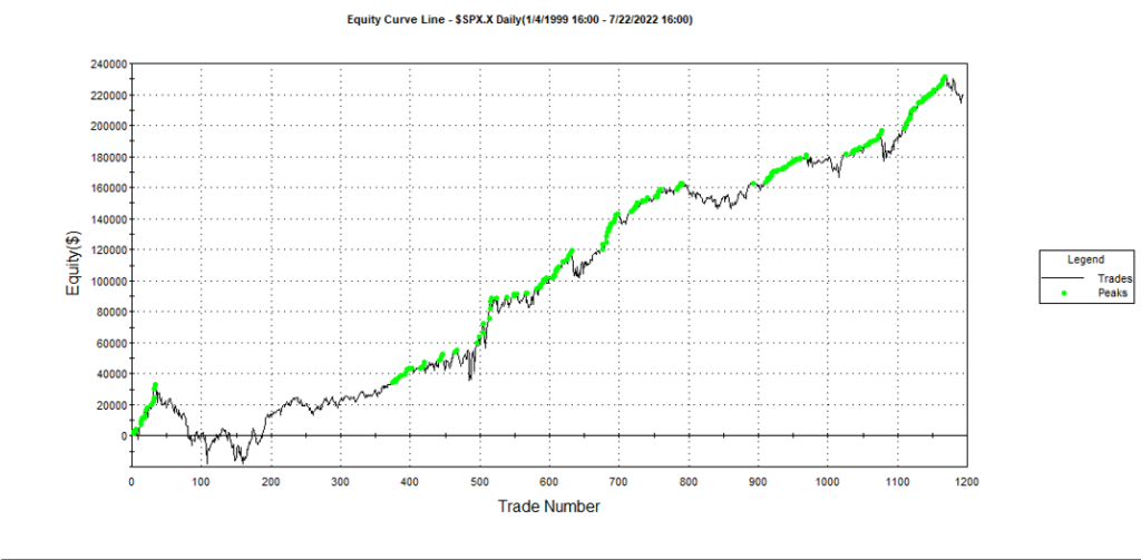
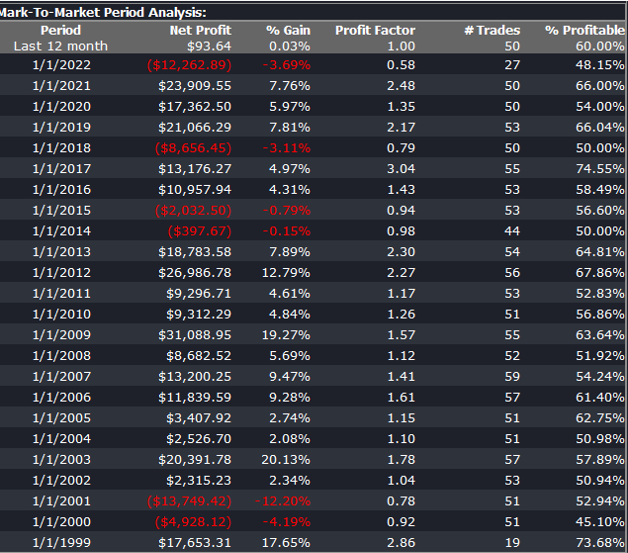
The strategy appears to work well “out-of-the-box”, i,e, without any further refinement. So our quest for a robust strategy appears to have been quite successful, given that none of the 23-year span of real market data on which the strategy was tested was used in the development process.

We can take the process a little further, however, by “optimizing” the strategy. Traditionally this would mean finding the optimal set of parameters that produces the highest net profit on the test data. But this would be curve fitting in the worst possible sense, and is not at all what I am suggesting.

Instead we use a procedure known as Walk Forward Optimization (WFO), as described in this post:

The goal of WFO is not to curve-fit the best parameters, which would entirely defeat the object of using synthetic data. Instead, its purpose is to test the robustness of the strategy. We accomplish this by using a sequence of overlapping in-sample and out-of-sample periods to evaluate how well the strategy stands up, assuming the parameters are optimized on in-sample periods of varying size and start date and tested of similarly varying out-of-sample periods. A strategy that fails a cluster of such tests is unlikely to prove robust in live trading. A strategy that passes a test cluster at least demonstrates some capability to perform well in different market regimes.

To some extent we might regard such a test as unnecessary, given that the strategy has already been observed to perform well under several different market conditions, encapsulated in the different synthetic price series, in addition to the real historical price series. Nonetheless, we conduct a WFO cluster test to further evaluate the robustness of the strategy.

As the goal of the procedure is not to maximize the theoretical profitability of the strategy, but rather to evaluate its robustness, we select a criterion other than net profit as the factor to optimize. Specifically, we select the sum of the areas of the strategy drawdowns as the quantity to minimize (by maximizing the inverse of the sum of drawdown areas, which amounts to the same thing). This requires a little explanation.

If we look at the strategy drawdown periods of the equity curve, we observe several periods (highlighted in red) in which the strategy was underwater:
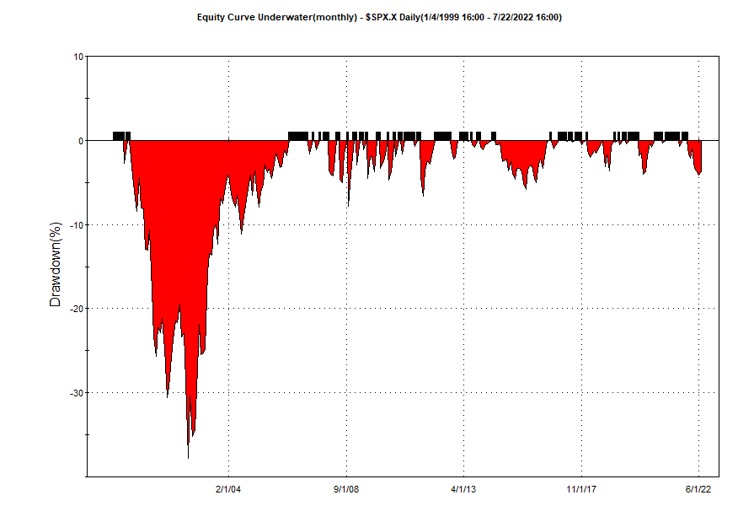
The area of each drawdown represents the length and magnitude of the drawdown and our goal here is to minimize the sum of these areas, so that we reduce both the total duration and severity of strategy drawdowns.

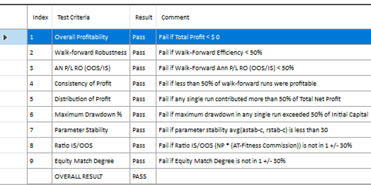
In each WFO test we use different % of OOS data and a different number of runs, assessing the performance of the strategy on a battery of different criteria:
x

These criteria not only include overall profitability, but also factors such as parameter stability, profit consistency in each test, the ratio of in-sample to out-of-sample profits, etc. In other words, this WFO cluster analysis is not about profit maximization, but robustness evaluation, as assessed by these several different metrics. And in this case the strategy passes every test with flying colors:
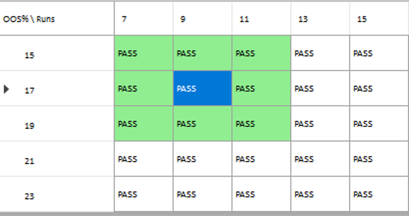
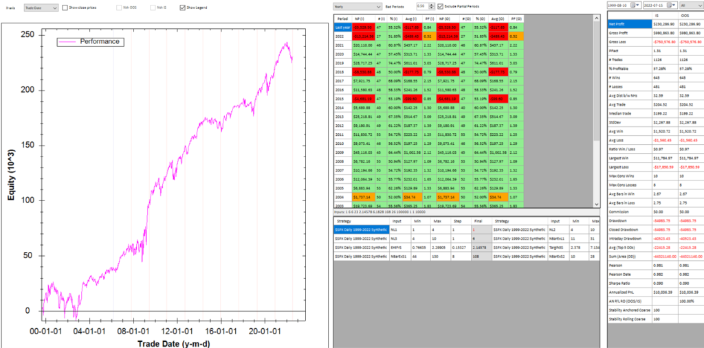
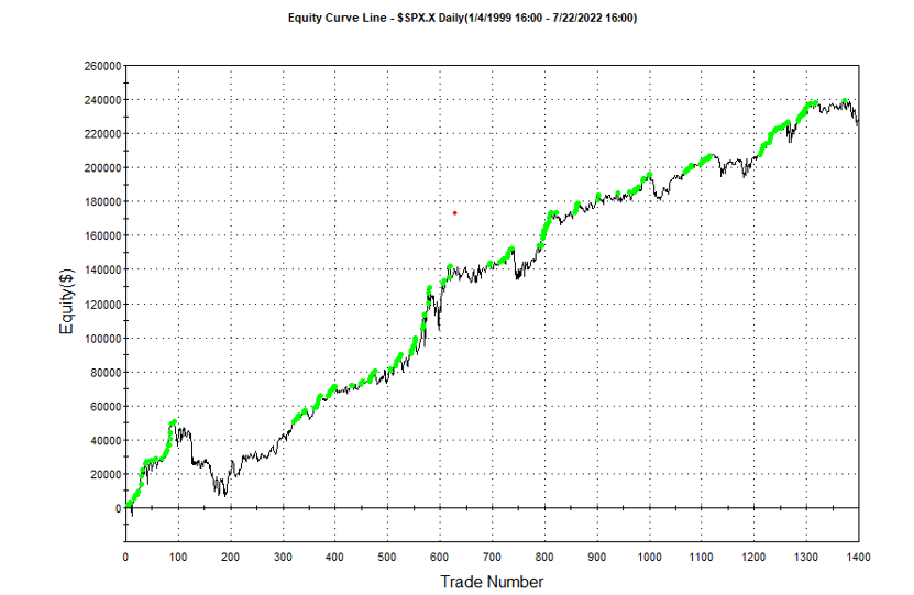
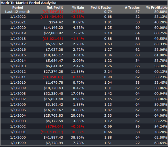
Other than validating the robustness of the strategy’s performance, the overall effect of the procedure is to slightly improve the equity curve by diminishing the magnitude and duration of the drawdown periods:
Conclusion

We have shown how, by using synthetic price series, we can build a robust trading strategy that performs well under a variety of different market conditions, including on previously “unseen” historical market data. Further analysis using cluster WFO tests strengthens the assessment of the strategy’s robustness.

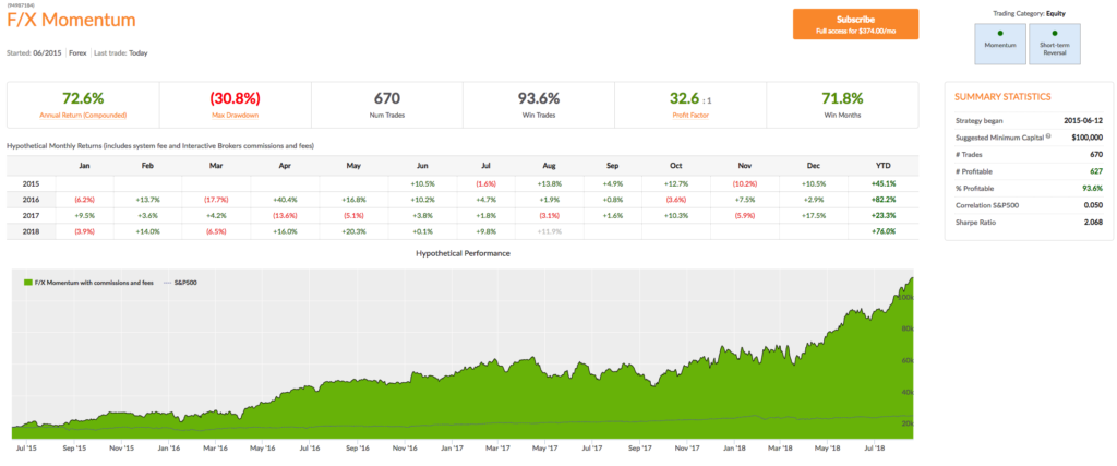
The F/X Momentum Strategy

Our approach is based upon the idea that currencies tend to be range bound, that momentum ultimately exhausts itself and that prices tend to fall faster than they rise. The strategy seeks to exploit these characteristics with short trades that may be closed within a few hours, or continue over several days when the exhaustion pattern emerges more slowly.
FXMomentum Aug 20 2018

Career Opportunity for Quant Traders

Career Opportunity for Quant Traders as Strategy Managers

We are looking for 3-4 traders (or trading teams) to showcase as Strategy Managers on our Algorithmic Trading Platform.  Ideally these would be systematic quant traders, since that is the focus of our fund (although they don’t have to be).  So far the platform offers a total of 10 strategies in equities, options, futures and f/x.  Five of these are run by external Strategy Managers and five are run internally.

The goal is to help Strategy Managers build a track record and gain traction with a potential audience of over 100,000 members.  After a period of 6-12 months we will offer successful managers a position as a PM at Systematic Strategies and offer their strategies in our quantitative hedge fund.  Alternatively, we will assist the manager is raising external capital in order to establish their own fund.

If you are interested in the possibility (or know a talented rising star who might be), details are given below.

Manager Platform

Volatility Trading Styles

The VIX Surge of Feb 2018

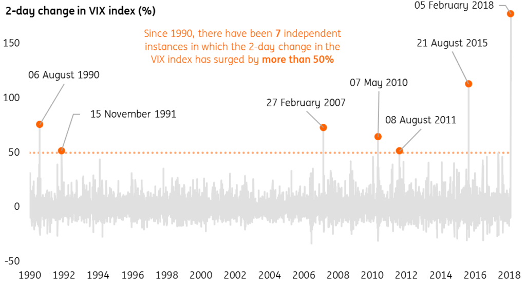
Volatility trading has become a popular niche in investing circles over the last several years.  It is easy to understand why:  with yields at record lows it has been challenging to find an alternative to equities that offers a respectable return.  Volatility, however, continues to be volatile (which is a good thing in this context) and the steepness of the volatility curve has offered investors attractive returns by means of the volatility carry trade.  In this type of volatility trading the long end of the vol curve is sold, often using longer dated futures in the CBOE VIX Index, for example.  The idea is that profits are generated as the contract moves towards expiration, “riding down” the volatility curve as it does so.  This is a variant of the ever-popular “riding down the yield curve” strategy, a staple of fixed income traders for many decades.  The only question here is what to use to hedge the short volatility exposure – highly correlated S&P500 futures are a popular choice, but the resulting portfolio is exposed to significant basis risk.  Besides, when the volatility curve flatten and inverts, as it did in spectacular fashion in February, the transition tends to happen very quickly, producing a substantial losses on the portfolio.  These may be temporary, if the volatility spike is small or short-lived, but as traders and investors discovered in the February drama, neither of these two desirable outcomes is guaranteed.  Indeed as I pointed out in an earlier post this turned out to be the largest ever two-day volatility surge in history.  The results for many hedge funds, especially in the quant sector were devastating, with several showing high single digit or double-digit losses for the month.

VIX_Spike_1


Over time, investors have become more familiar with the volatility space and have learned to be wary of strategies like volatility carry or option selling, where the returns look superficially attractive, until a market event occurs.  So what alternative approaches are available?

An Aggressive Approach to Volatility Trading

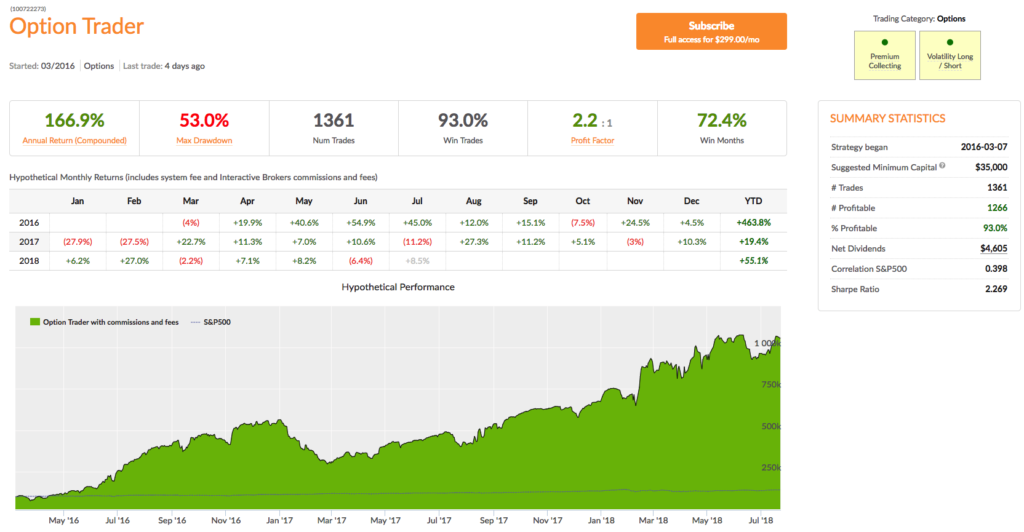
In my blog post Riders on the Storm  I described one such approach:  the Option Trader strategy on our Algo Trading Platform made a massive gain of 27% for the month of February and as a result strategy performance is now running at over 55% for 2018 YTD, while maintaining a Sharpe Ratio of 2.23.

Option Trader


The challenge with this style of volatility trading is that it requires a trader (or trading system) with a very strong stomach and an investor astute enough to realize that sizable drawdowns are in a sense “baked in” for this trading strategy and should be expected from time to time.  But traders are often temperamentally unsuited to this style of trading – many react by heading for the hills and liquidating positions at the first sign of trouble; and the great majority of investors are likewise unable to withstand substantial drawdowns, even if the eventual outcome is beneficial.

SSALGOTRADING AD

The Market Timing Approach

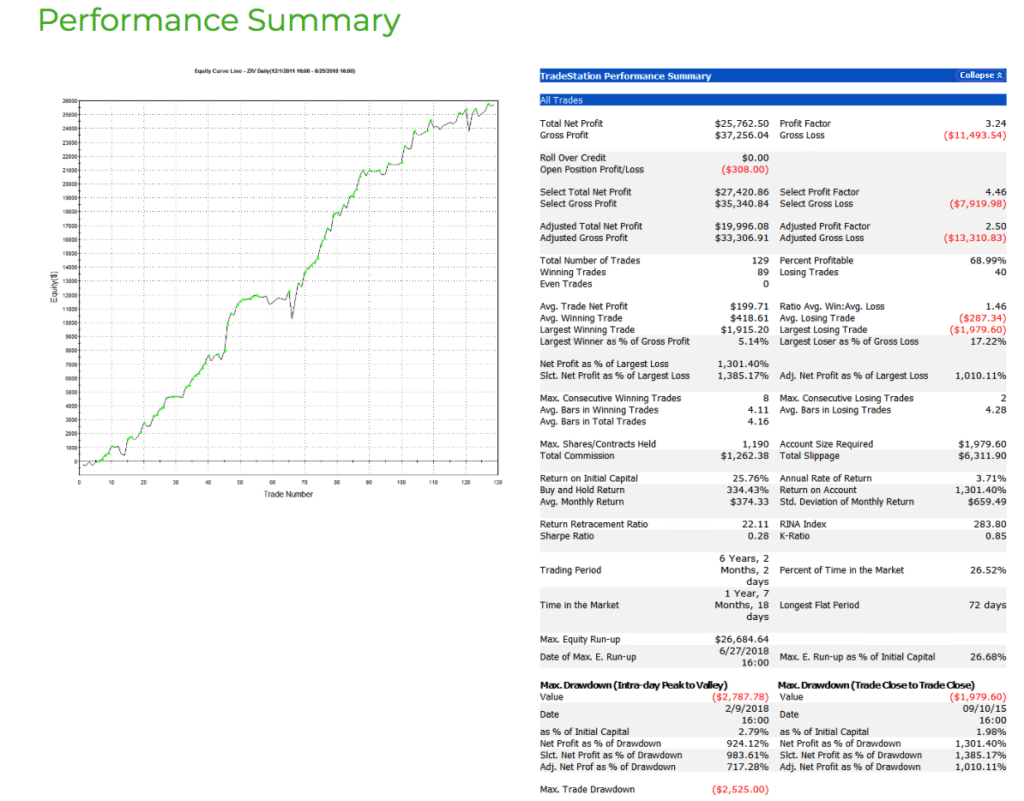
So what alternatives are there?  One way of dealing with the problem of volatility spikes is simply to try to avoid them.  That means developing a strategy logic that step aside altogether when there is a serious risk of an impending volatility surge.  Market timing is easy to describe, but very hard to implement successfully in practice.  The VIX Swing Trader strategy on the Systematic Algotrading platform attempts to do just that, only trading when it judges it safe to do so. So, for example, it completely side-stepped the volatility debacle in August 2015, ending the month up +0.74%.  The strategy managed to do the same in February this year, finishing ahead +1.90%, a pretty creditable performance given how volatility funds performed in general.  One helpful characteristic of the strategy is that it trades the less-volatile mid-section of the volatility curve, in the form of the VelocityShares Daily Inverse VIX MT ETN (ZIV).  This ensures that the P&L swings are much less dramatic than for strategies exposed to the front end of the curve, as most volatility strategies are.

VIX Swing Trader1 VIX Swing Trader2

A potential weakness of the strategy is that it will often miss great profit opportunities altogether, since its primary focus is to keep investors out of trouble. Allied to this, the system may trade only a handful of times each month.  Indeed, if you look at the track record above you find find months in which the strategy made no trades at all. From experience, investors are almost as bad at sitting on their hands as they are at taking losses:  patience is not a highly regarded virtue in the investing community these days.  But if you are a cautious, patient investor looking for a source of uncorrelated alpha, this strategy may be a good choice. On the other hand, if you are looking for high returns and are willing to take the associated risks, there are choices better suited to your goals.

The Hedging Approach to Volatility Trading

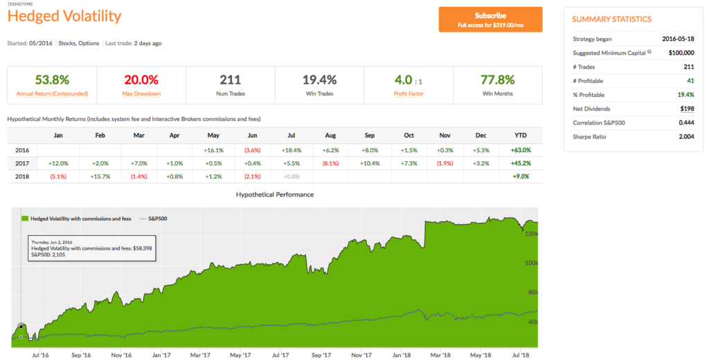
A “middle ground” is taken in our Hedged Volatility strategy. Like the VIX Swing Trader this strategy trades VIX ETFs/ETNs, but it does so across the maturity table. What distinguishes this strategy from the others is its use of long call options in volatility products like the iPath S&P 500 VIX ST Futures ETN (VXX) to hedge the short volatility exposure in other ETFs in the portfolio.  This enables the strategy to trade much more frequently, across a wider range of ETF products and maturities, with the security of knowing that the tail risk in the portfolio is protected.  Consequently, since live trading began in 2016, the strategy has chalked up returns of over 53% per year, with a Sharpe Ratio of 2 and Sortino Ratio above 3.  Don’t be confused by the low % of trades that are profitable:  the great majority of these loss-making “trades” are in fact hedges, which one would expect to be losers, as most long options trades are.  What matters is the overall performance of the strategy.

Hedged Volatility

All of these strategies are available on our Systematic Algotrading Platform, which offers investors the opportunity to trade the strategies in their own brokerage account for a monthly subscription fee.

The Multi-Strategy Approach

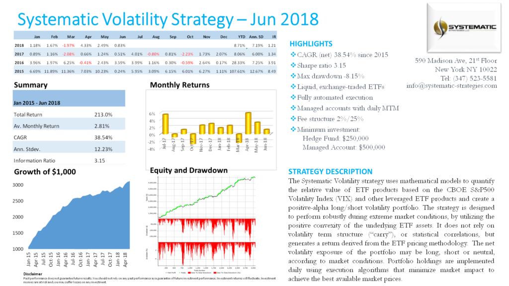
The approach taken by the Systematic Volatility Strategy in our Systematic Strategies hedge fund again seeks to steer a middle course between risk and return.  It does so by using a meta-strategy approach that dynamically adjusts the style of strategy deployed as market conditions change.  Rather than using options (the strategy’s mandate includes only ETFs) the strategy uses leveraged ETFs to provide tail risk protection in the portfolio. The strategy has produced an average annual compound return of 38.54% since live trading began in 2015, with a Sharpe Ratio of 3.15:

Systematic Volatility Strategy 1 Page Tear Sheet June 2018


A more detailed explanation of how leveraged ETFs can be used in volatility trading strategies is given in an earlier post:

http://jonathankinlay.com/2015/05/investing-leveraged-etfs-theory-practice/


Conclusion:  Choosing the Investment Style that’s Right for You

There are different styles of volatility trading and the investor should consider carefully which best suits his own investment temperament.  For the “high risk” investor seeking the greatest profit the Option Trader strategy in an excellent choice, producing returns of +176% per year since live trading began in 2016.   At the other end of the spectrum, the VIX Swing trader is suitable for an investor with a cautious trading style, who is willing to wait for the right opportunities, i.e. ones that are most likely to be profitable.  For investors seeking to capitalize on opportunities in the volatility space, but who are concerned about the tail risk arising from major market corrections, the Hedge Volatility strategy offers a better choice.  Finally, for investors able to invest $250,000 or more, a hedge fund investment in our Systematic Volatility strategy offers the highest risk-adjusted rate of return.

The New Long/Short Equity

High Frequency Trading Strategies

One of the benefits of high frequency trading strategies lies in their ability to produce risk-adjusted rates of return that are unmatched by anything that the hedge fund or CTA community is capable of producing.  With such performance comes another attractive feature of HFT firms – their ability to make money (almost) every day.  Of course, HFT firms are typically not required to manage billions of dollars, which is just as well given the limited capacity of most HFT strategies.  But, then again, with a Sharpe ratio of 10, who needs outside capital?  This explains why most investors have a difficult time believing the level of performance achievable in the high frequency world – they never come across such performance, because HFT firms generally have little incentive to show their results to external investors.

SSALGOTRADING AD

By and large, HFT strategies remain the province of proprietary trading firms that can afford to make an investment in low-latency trading infrastructure that far exceeds what is typically required for a regular trading or investment management firm.  However, while the highest levels of investment performance lie beyond the reach of most investors and money managers, it is still possible to replicate some of the desirable characteristics of high frequency strategies.

Quantitative Equity Strategy

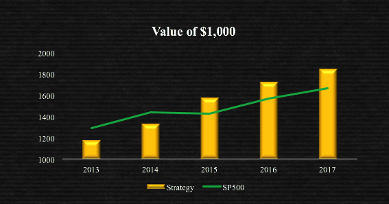
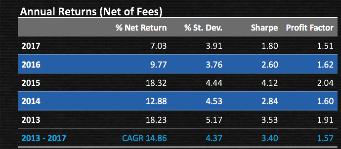
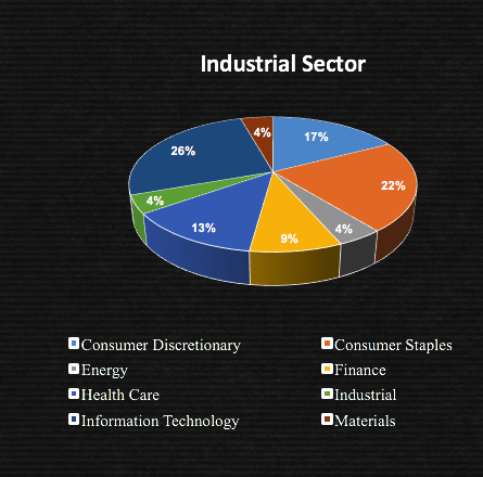
I am going to use an example our Quantitative Equity strategy, which forms part of the Systematic Strategies hedge fund.  The tables and charts below give a broad impression of the performance characteristics of the strategy, which include a CAGR of 14.85% (net of fees) since live trading began in 2013.

Value $1000
The NewEquityLSFig3


This is a strategy that is designed to produce returns on a  par with the S&P 500 index, but with considerably lower risk:  at just over 4%, the annual volatility of the strategy is only around 1/3 that of the index, while the maximum drawdown has been a little over 2% since inception.  This level of portfolio risk is much lower than can typically be achieved in an equity long/short strategy  (equity market neutral is another story, of course). Furthermore, the realized information ratio of 3.4 is in the upper 1%-tile of risk-adjusted performance amongst equity long/short strategies.  So something rather more interesting must be going on that is very different from the typical approach to long/short equity.
TheNewEquityLSFig5


One plausible explanation is that the strategy is exploiting some minor market anomaly that works fine for small amounts of capital, but which cannot be scaled.  But this is not the case here:  the investment universe comprises more than a hundred of the most liquid stocks in US markets, across a broad spectrum of sectors.  And while single-name investment is capped at 10% of average daily volume, this nonetheless provides investment capacity of several hundreds of millions of dollars.

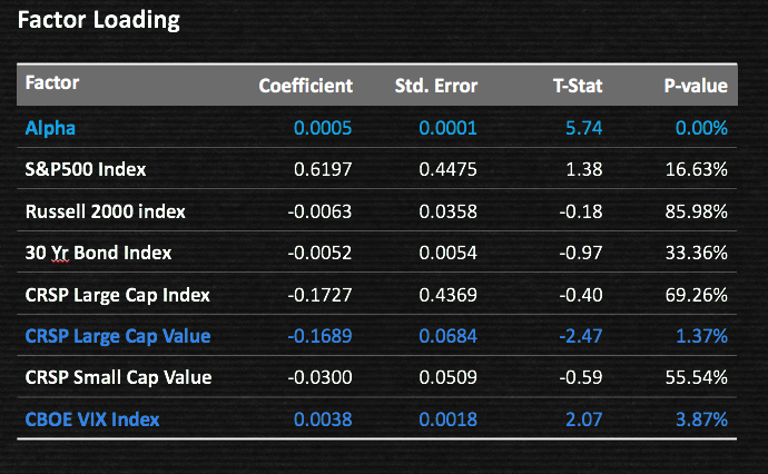
Nor does the reason for the exceptional performance lie in some new portfolio construction technique:  rather, we rely on a straightforward 1/n allocation.  Again, neither is factor exposure the driver of strategy alpha:  as the factor loading table illustrates, strategy performance is largely uncorrelated with most market indices.  It loads significantly on only large cap value, chiefly because the investment universe is defined as comprising the stocks with greatest liquidity (which tend to be large cap value), and on the CBOE VIX index.  The positive correlation with market volatility is a common feature of many types of trading strategy that tend to do better in volatile markets, when short-term investment opportunities are plentiful.

FactorLoadings

While the detail of the strategy must necessarily remain proprietary, I can at least offer some insight that will, I hope, provide food for thought.

We can begin by comparing the returns for two of the stocks in the portfolio, Home Depot and Pfizer.  The charts demonstrate one of important strategy characteristic: not every stock is traded at the same frequency.  Some stocks might be traded once or twice a month; others possibly ten times a day, or more.  In other words, the overall strategy is diversified significantly, not only across assets, but also across investment horizons.  This has a considerable impact on volatility and downside risk in the portfolio.

Home Depot vs. Pfizer Inc.

HD

PFEOverall, the strategy trades an average of 40-60 times a day, or more.   This is, admittedly, towards the low end of the frequency spectrum of HFT strategies – we might describe it as mid-frequency rather than high frequency trading.  Nonetheless,  compared to traditional long/short equity strategies this constitutes a high level of trading activity which, in aggregate, replicates some of the time-diversification benefits of HFT strategies, producing lower strategy volatility.

There is another way in which the strategy mimics, at least partially, the characteristics of a HFT strategy.  The profitability of many (although by no means all) HFT strategies lies in their ability to capture (or, at least, not pay) the bid-offer spread.  That is why latency is so crucial to most HFT strategies – if your aim is to to earn rebates, and/or capture the spread, you must enter and  exit, passively, often using microstructure models to determine when to lean on the bid or offer price.  That in turn depends on achieving a high priority for your orders in the limit order book, which is a function of  latency – you need to be near the top of the queue at all times in order the achieve the required fill rate.

How does that apply here?  While we are not looking to capture the spread, the strategy does seek to avoid taking liquidity and paying the spread.  Where it can do so,  it will offset the bid-offer spread by earning rebates.  In many cases we are able to mitigate the spread cost altogether.  So, while it cannot accomplish what a HFT market-making system can achieve, it can mimic enough of its characteristics – even at low frequency – to produce substantial gains in terms of cost-reduction and return enhancement.  This is important since the transaction volume and portfolio turnover in this approach are significantly greater than for a typical equity long/short strategy.

Portfolio of Strategies vs. Portfolio of Equities

slide06But this feature, while important, is not really the heart of the matter.  Rather, the central point is this:  that the overall strategy is an assembly of individual, independent strategies for each component stock.  And it turns out that the diversification benefit of a portfolio of strategies is generally far greater than for an equal number of stocks, because the equity processes themselves will typically be correlated to a far greater degree than will corresponding trading strategies.  To take the example of the pair of stocks discussed earlier, we find that the correlation between HD and PFE over the period from 2013 to 2017 is around 0.39, based on daily returns.  By comparison, the correlation between the strategies for the two stocks over the same period is only 0.01.

This is generally the case, so that a portfolio of, say, 30 equity strategies, might reasonably be expected to enjoy a level of risk that is perhaps as much as one half that of a portfolio of the underlying stocks, no matter how constructed.  This may be due to diversification in the time dimension, coupled with differences in the alpha generation mechanisms of the underlying strategies – mean reversion vs. momentum, for example

Strategy Robustness Testing

There are, of course, many different aspects to our approach to strategy risk management. Some of these are generally applicable to strategies of all varieties, but there are others that are specific to this particular type of strategy.

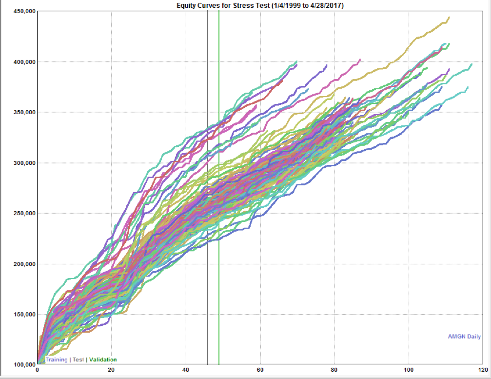
A good example of the latter is how we address the issue of strategy robustness. One of the principal concerns that investors have about quantitive strategies is that they may under-perform during adverse market conditions, or even simply stop working altogether. Our approach is to stress test each of the sub-strategy models using Monte Carlo simulation and examine their performance under a wide range of different scenarios, many of which have never been seen in the historical data used to construct the models.
For instance, we typically allow prices to fluctuate randomly by +/- 30% from historical values. But we also randomize the start date of each strategy by up to a year, which reduces the likelihood of a strategy being selected simply on the strength of a lucky start. Finally, we are interested in ensuring that the performance of each sub-strategy is not overly sensitive to the specific parameter values chosen for each model. Again, we test this using Monte Carlo, assessing the performance of each sub-strategy if the parameter values of the model are varied randomly by up to 30%.

The output of all these simulation tests is compiled into a histogram of performance results, from which we select the worst 5%-tile. Only if the worst outcomes – the 1-in-20 results in the left tail of the performance distribution – meet our performance criteria will the sub-strategy advance to the next stage of evaluation, simulated trading. This gives us – and investors – a level of confidence in the ability of the strategy to continue to perform well regardless of how market conditions evolve over time.

MonteCarlo Stress test


An obvious question to ask at this point is: if this is such a great idea, why don’t more firms use this approach?  The answer is simple: it involves too much research.  In a typical portfolio strategy there is a single investment idea that is applied cross-sectionally to a universe of stocks (factor models, momentum models, etc).  In the strategy portfolio approach, separate strategies must be developed for each stock individually, which takes far more time and effort.  Consequently such strategies must necessarily scale more slowly.

Another downside to the strategy portfolio approach is that it is less able to control the portfolio characteristics.  For instance, the overall portfolio may, on average, have a beta close to zero; but there are likely to be times when a majority of the individual stock strategies align, producing a significantly higher, or lower, beta.  The key here is to ask the question: what matters more – the semblance of risk control, or the actual risk characteristics of the strategy?  In reality, the risk controls of traditional long/short equity strategies often turn out to be more theoretical than real.  Time and again investors have seen strategies that turn out to be downside-correlated with the market, regardless of the purported “market-neutral” characteristics of the portfolio.  I would argue that what matters far more is how the strategy actually performs under conditions of market stress, regardless of how “market neutral” or “sector neutral” it may purport to be.  And while I agree that this is hardly a widely-held view, my argument would be that one cannot expect to achieve above-average performance simply by employing standard approaches at every turn.

Parallels with Fund of Funds Investment

So, is this really a “new approach” to equity long/short? Actually, no.  It is certainly unusual.  But it follows quite closely the model of a proprietary trading firm, or a Fund of Funds. There, as here, the task is to create a combined portfolio of strategies (or managers), rather than by investing directly in the underlying assets.  A Fund of Funds will seek to create a portfolio of strategies that have low correlations to one another, and may operate a meta-strategy for allocating capital to the component strategies, or managers.  But the overall investment portfolio cannot be as easily constrained as an individual equity portfolio can be – greater leeway must be allowed for the beta, or the dollar imbalance in the longs and shorts, to vary from time to time, even if over the long term the fluctuations average out.  With human managers one always has to be concerned about the risk of “style drift” – i.e. when managers move away from their stated investment mandate, methodologies or objectives, resulting in a different investment outcomes.  This can result in changes in the correlation between a strategy and its peers, or with the overall market.  Quantitative strategies are necessarily more consistent in their investment approach – machines generally don’t alter their own source code – making a drift in style less likely.  So an argument can be made that the risk inherent in this form of equity long/short strategy is on a par with – certainly not greater than – that of a typical fund of funds.

Conclusions

An investment approach that seeks to create a portfolio of strategies, rather than of underlying assets, offers a significant advantage in terms of risk reduction and diversification, due to the relatively low levels of correlation between the component strategies.   The trading costs associated with higher frequency trading can be mitigated using passive entry/exit rules designed to avoid taking liquidity and generating exchange rebates.  The downside is that it is much harder to manage the risk attributes of the portfolio, such as the portfolio beta, sector risk, or even the overall net long/short exposure.  But these are indicators of strategy risk, rather than actual risk itself and they often fail to predict the actual risk characteristics of the strategy, especially during conditions of market stress.  Investors may be better served by an approach to long/short equity that seeks to maximize diversification on the temporal axis as well as in terms of the factors driving strategy alpha.


Disclaimer: past performance does not guarantee future results. You should not rely on any past performance as a guarantee of future investment performance. Investment returns will fluctuate. Investment monies are at risk and you may suffer losses on any investment.

Machine Learning Trading Systems

The SPDR S&P 500 ETF (SPY) is one of the widely traded ETF products on the market, with around $200Bn in assets and average turnover of just under 200M shares daily.  So the likelihood of being able to develop a money-making trading system using publicly available information might appear to be slim-to-none. So, to give ourselves a fighting chance, we will focus on an attempt to predict the overnight movement in SPY, using data from the prior day’s session.

In addition to the open/high/low and close prices of the preceding day session, we have selected a number of other plausible variables to build out the feature vector we are going to use in our machine learning model:

  • The daily volume
  • The previous day’s closing price
  • The 200-day, 50-day and 10-day moving averages of the closing price
  • The 252-day high and low prices of the SPY series

We will attempt to build a model that forecasts the overnight return in the ETF, i.e.  [O(t+1)-C(t)] / C(t)

SSALGOTRADING AD

In this exercise we use daily data from the beginning of the SPY series up until the end of 2014 to build the model, which we will then test on out-of-sample data running from Jan 2015-Aug 2016.  In a high frequency context a considerable amount of time would be spent evaluating, cleaning and normalizing the data.  Here we face far fewer problems of that kind.  Typically one would standardized the input data to equalize the influence of variables that may be measured on scales of very different orders of magnitude.  But in this example all of the input variables, with the exception of volume, are measured on the same scale and so standardization is arguably unnecessary.

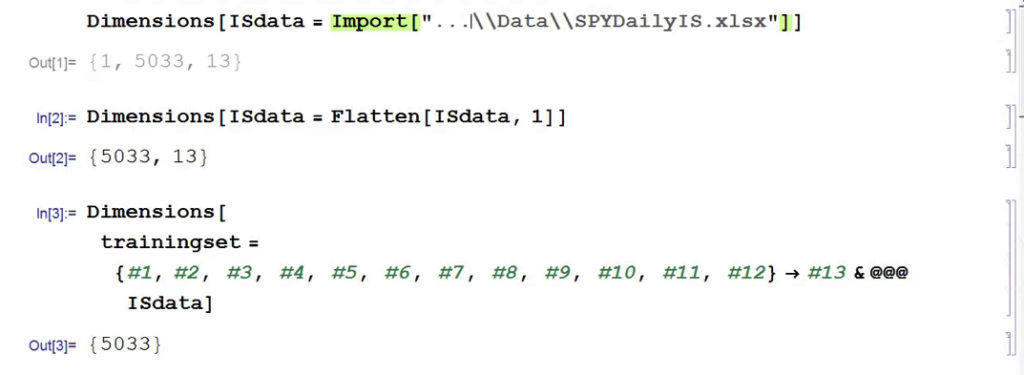
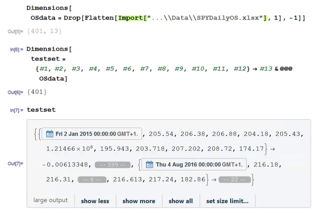
First, the in-sample data is loaded and used to create a training set of rules that map the feature vector to the variable of interest, the overnight return:


fig1


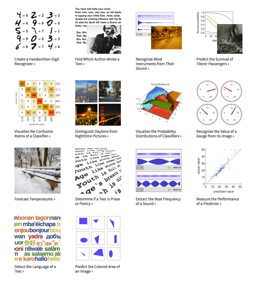
In Mathematica 10 Wolfram introduced a suite of machine learning algorithms that include regression, nearest neighbor, neural networks and random forests, together with functionality to evaluate and select the best performing machine learning technique.  These facilities make it very straightfoward to create a classifier or prediction model using machine learning algorithms, such as this handwriting recognition example:

handwriting

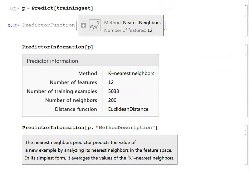
We create a predictive model on the SPY trainingset, allowing Mathematica to pick the best machine learning algorithm:

fig3

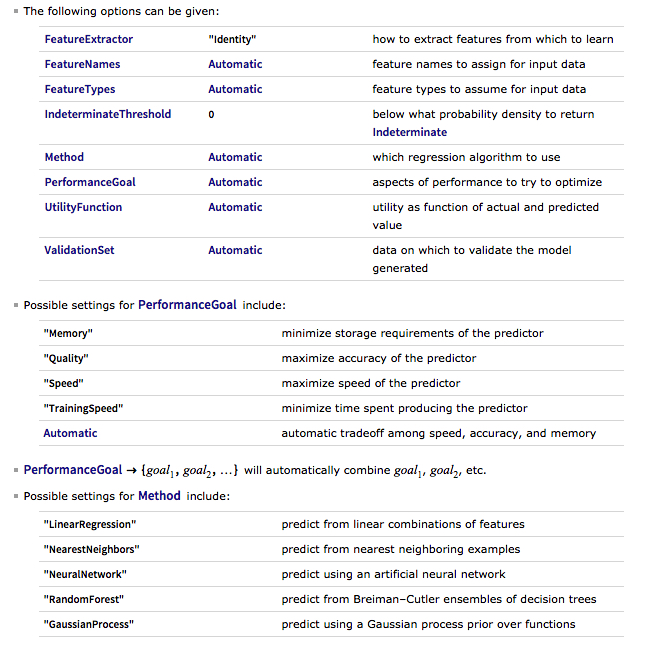
There are a number of options for the Predict function that can be used to control the feature selection, algorithm type, performance type and goal, rather than simply accepting the defaults, as we have done here:

fig4

Having built our machine learning model, we load the out-of-sample data from Jan 2015 to Aug 2016, and create a test set:

fig5


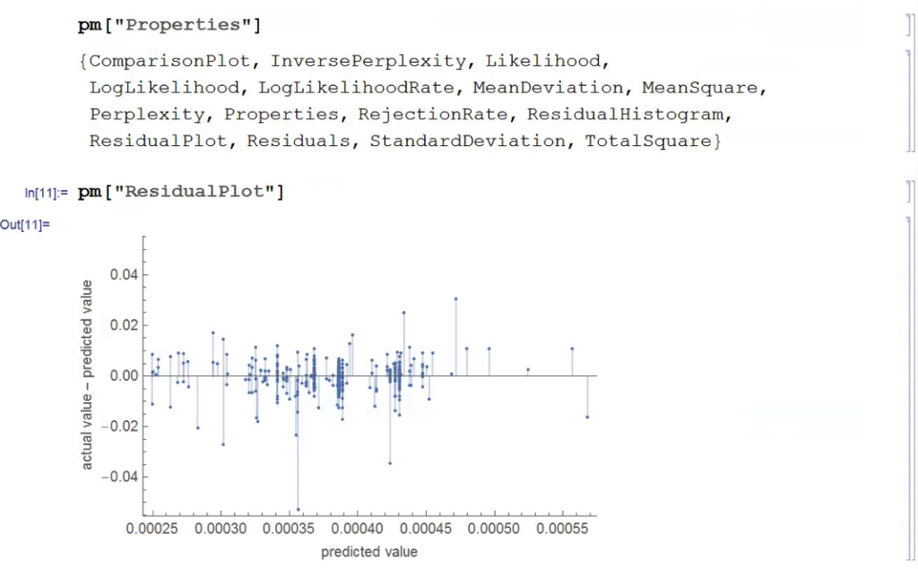
We next create a PredictionMeasurement object,  using the Nearest Neighbor model , that can be used for further analysis:


fig6

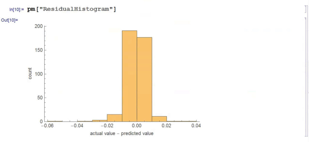
fig7

fig8


There isn’t much dispersion in the model forecasts, which all have positive value.  A common technique in such cases is to subtract the mean from each of the forecasts (and we may also standardize them by dividing by the standard deviation).

The scatterplot of actual vs. forecast overnight returns in SPY now looks like this:

scatterplot


There’s still an obvious lack of dispersion in the forecast values, compared to the actual overnight returns, which we could rectify by standardization. In any event, there appears to be a small, nonlinear relationship between forecast and actual values, which holds out some hope that the model may yet prove useful.

From Forecasting to Trading

There are various methods of deploying a forecasting model in the context of creating a trading system.  The simplest route, which we  will take here, is to apply a threshold gate and convert the filtered forecasts directly into a trading signal. But other approaches are possible, for example:

  • Combining the forecasts from multiple models to create a prediction ensemble
  • Using the forecasts as inputs to a genetic programming model
  • Feeding the forecasts into the input layer of  a neural network model designed specifically to generate trading signals, rather than forecasts

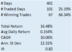
In this example we will create a trading model by applying a simple filter to the forecasts, picking out only those values that exceed a specified threshold. This is a standard trick used to isolate the signal in the model from the background noise.  We will accept only the positive signals that exceed the threshold level, creating a long-only trading system.  i.e. we ignore forecasts that fall below the threshold level.  We buy SPY at the close when the forecast exceeds the threshold and exit any long position at the next day’s open.  This strategy produces the following pro-forma results:


Perf table


equity curve


Conclusion

The system has some quite attractive features, including a win rate of over 66%  and a CAGR of over 10% for the out-of-sample period.

Obviously, this is a very basic illustration: we would want to factor in trading commissions, and the slippage incurred entering and exiting positions in the post- and pre-market periods, which will negatively impact performance, of course.  On the other hand, we have barely begun to scratch the surface in terms of the variables that could be considered for inclusion in the feature vector, and which may increase the explanatory power of the model.

In other words, in reality, this is only the beginning of a lengthy and arduous research process. Nonetheless, this simple example should be enough to give the reader a taste of what’s involved in building a predictive trading model using machine learning algorithms.