

Amongst a wide variety of money management methods that have evolved over the years, a perennial favorite is the use of the equity curve to guide position sizing. The most common version of this technique is to add to the existing position (whether long or short) depending on the relationship between the current value of the account equity (realized + unrealized PL) and its moving average. According to whether you believe that the equity curve is momentum driven, or mean reverting, you will add to your existing position when the equity move above (or, on the case of mean-reverting, below) the long term moving average.
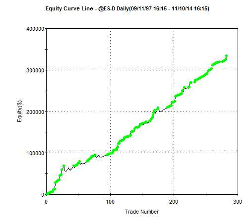
In this article I want to discuss a slightly different version of equity curve money management, which is mean-reversion oriented. The underlying thesis is that your trading strategy has good profit characteristics, and while it suffers from the occasional, significant drawdown, it can be expected to recover from the downswings. You should therefore be looking to add to your positions when the equity curve moves down sufficiently, in the expectation that the trading strategy will recover. The extra contracts you add to your position during such downturns with increase the overall P&L. To illustrate the approach I am going to use a low frequency strategy on the S&P500 E-mini futures contract (ES). The performance of the strategy is summarized in the chart and table below. 
(click to enlarge)
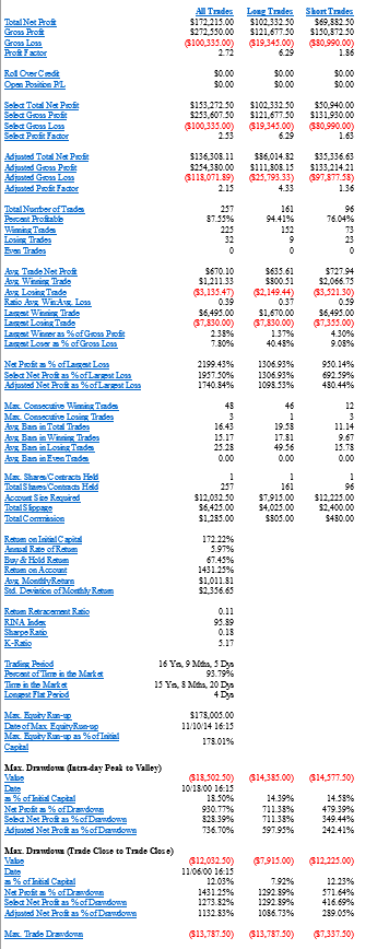
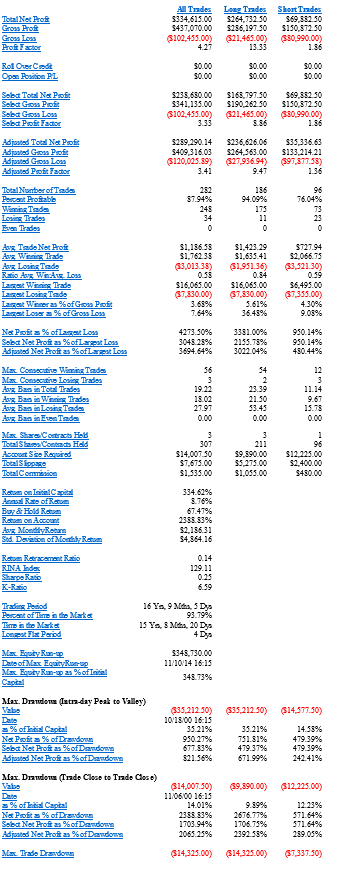
The overall results of the strategy are not bad: at over 87% the win rate is high as, too, is the profit factor of 2.72. And the strategy’s performance, although hardly stellar, has been quite consistent over the period from 1997. That said, most the profits derive from the long side, and the strategy suffers from the occasional large loss, including a significant drawdown of over 18% in 2000.
I am going to use this underlying strategy to illustrate how its performance can be improved with equity curve money management (ECMM). To start, we calculate a simple moving average of the equity curve, as before. However, in this variation of ECMM we then calculate offsets that are a number of standard deviations above or below the moving average. Typical default values for the moving average length might be 50 bars for a daily series, while we might use, say, +/- 2 S.D. above and below the moving average as our trigger levels. The idea is that we add to our position when the equity curve falls below the lower threshold level (moving average – 2x S.D) and then crosses back above it again. This is similar to how a trader might use Bollinger bands, or an oscillator like Stochastics. The chart below illustrates the procedure.
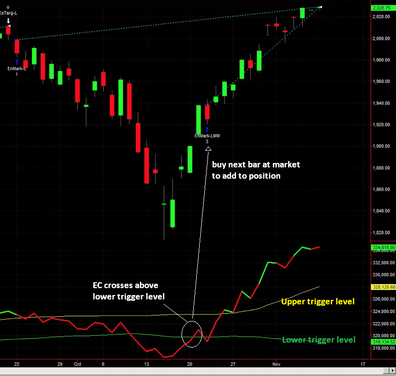
The lower and upper trigger levels are shown as green and yellow lines in the chart indicator (note that in this variant of ECMM we only use the lower level to add to positions).
After a significant drawdown early in October the equity curve begins to revert and crosses back over the lower threshold level on Oct 21. Applying our ECMM rule, we add to our existing long position the next day, Oct 22 (the same procedure would apply to adding to short positions). As you can see, our money management trade worked out very well, since the EC did continue to mean-revert as expected. We closed the trade on Nov 11, for a substantial, additional profit.
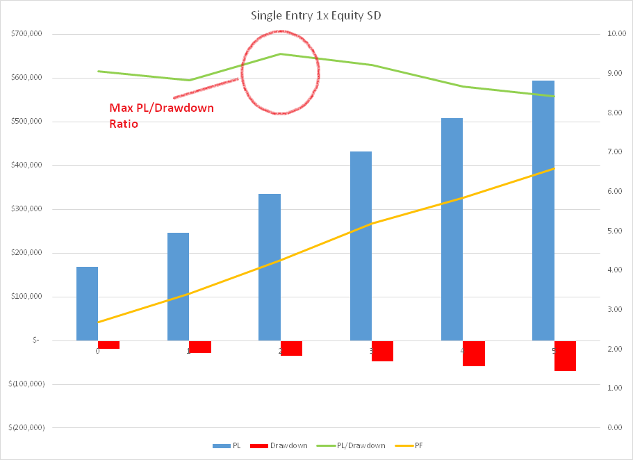
Now we have illustrated the procedure, let’s being to explore the potential of the ECMM idea in more detail. The first important point to understand is what ECMM will NOT do: i.e. reduce risk. Like all money management techniques that are designed to pyramid into positions, ECMM will INCREASE risk, leading to higher drawdowns. But ECMM should also increase profits: so the question is whether the potential for greater profits is sufficient to offset the risk of greater losses. If not, then there is a simpler alternative method of increasing profits: simply increase position size! It follows that one of the key metrics of performance to focus on in evaluating this technique is the ratio of PL to drawdown. Let’s look at some examples for our baseline strategy.
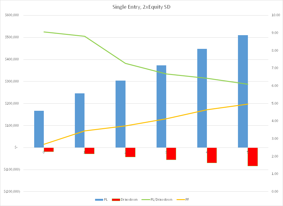
The chart shows the effect of adding a specified number of contracts to our existing long or short position whenever the equity curve crosses back above the lower trigger level, which in this case is set at 2xS.D below the 50-day moving average of the equity curve. As expected, the overall strategy P&L increases linearly in line with the number of additional contracts traded, from a base level of around $170,000, to over $500,000 when we trade an additional five contracts. So, too, does the profit factor rise from around 2.7 to around 5.0. That’s where the good news ends. Because, just as the strategy PL increases, so too does the size of the maximum drawdown, from $(18,500) in the baseline case to over $(83,000) when we trade an additional five contracts. In fact, the PL/Drawdown ratio declines from over 9.0 in the baseline case, to only 6.0 when we trade the ECMM strategy with five additional contracts. In terms of risk and reward, as measured by the PL/Drawdown ratio, we would be better off simply trading the baseline strategy: if we traded 3 contracts instead of 1 contract, then without any money management at all we would have made total profits of around $500,000, but with a drawdown of just over $(56,000). This is the same profit as produced with the 5-contract ECMM strategy, but with a drawdown that is $23,000 smaller.

How does this arise? Quite simply, our ECMM money management trades as not all automatic winners from the get-go (even if they eventually produce profits. In some cases, having crossed above the lower threshold level, the equity curve will subsequently cross back down below it again. As it does so, the additional contracts we have traded are now adding to the strategy drawdown.
This suggests that there might be a better alternative. How about if, instead of doing a single ECMM trade for, say, 5 additional contracts, we instead add an additional contract each time the equity curve crosses above the lower threshold level. Sure, we might give up some extra profits, but our drawdown should be lower, right? That turns out to be true. Unfortunately, however, profits are impacted more than the drawdown, so as a result the PL/Drawdown ratio shows the same precipitous decline:
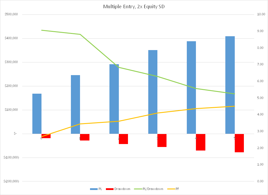
Once again, we would be better off trading the baseline strategy in larger size, rather than using ECMM, even when we scale into the additional contracts.
What else can we try? An obvious trick to try is tweaking the threshold levels. We can do this by adjusting the # of standard deviations at which to set the trigger levels. Intuitively, it might seem that the obvious thing to do is set the threshold levels further apart, so that ECMM trades are triggered less frequently. But, as it turns out, this does not produce the desired effect. Instead, counter-intuitively, we have to set the threshold levels CLOSER to the moving average, at only +/-1x S.D. The results are shown in the chart below.
With these settings, the strategy PL and profit factor increase linearly, as before. So too does the strategy drawdown, but at a slower rate. As a consequence, the PL/Drawdown ration actually RISES, before declining at a moderate pace. Looking at the chart, it is apparent the optimal setting is trading two additional contracts with a threshold setting one standard deviation below the 50-day moving average of the equity curve.
Below are the overall results. With these settings the baseline strategy plus ECMM produces total profits of $334,000, a profit factor of 4.27 and a drawdown of $(35,212), making the PL/Drawdown ratio 9.50. Producing the same rate of profits using the baseline strategy alone would require us to trade two contracts, producing a slightly higher drawdown of almost $(37,000). So our ECMM strategy has increased overall profitability on a risk-adjusted basis.
(Click to enlarge)
CONCLUSION
It is certainly feasible to improve not only the overall profitability of a strategy using equity curve money management, but also the risk-adjusted performance. Whether ECMM will have much effect depends on the specifics of the underlying strategy, and the level at which the ECMM parameters are set to. These can be optimized on a walk-forward basis.
EASYLANGUAGE CODE
Inputs:
MALen(50),
SDMultiple(2),
PositionMult(1),
ExitAtBreakeven(False);
Var:
OpenEquity(0),
EquitySD(0),
EquityMA(0),
UpperEquityLevel(0),
LowerEquityLevel(0),
NShares(0);
OpenEquity=OpenPositionProfit+NetProfit;a
EquitySD=stddev(OpenEquity,MALen);
EquityMA=average(OpenEquity,MALen);
UpperEquityLevel=EquityMA + SDMultiple*EquitySD;
LowerEquityLevel=EquityMA-SDMultiple*EquitySD;
NShares=CurrentContracts*PositionMult;
If OpenEquity crosses above LowerEquityLevel then begin
If Marketposition > 0 then begin
Buy(“EnMark-LMM”) NShares shares next bar at market;
end;
If Marketposition < 0 then begin
Sell Short(“EnMark-SMM”) NShares shares next bar at market;
end;
end;
If ExitAtBreakeven then begin
If OpenEquity crosses above EquityMA then begin
If Marketposition > 1 then begin
Sell Short (“ExBE-LMM”) (Currentcontracts-1) shares next bar at market;
end;
If Marketposition < -1 then begin
Buy (“ExBE-SMM”) (Currentcontracts-1) shares next bar at market;
end;
end;
end;