Volatility Forecasting in Emerging Markets

The great majority of empirical studies have focused on asset markets in the US and other developed economies.   The purpose of this research is to determine to what extent the findings of other researchers in relation to the characteristics of asset volatility in developed economies applies also to emerging markets.  The important characteristics observed in asset volatility that we wish to identify and examine in emerging markets include clustering, (the tendency for periodic regimes of high or low volatility) long memory, asymmetry, and correlation with the underlying returns process.  The extent to which such behaviors are present in emerging markets will serve to confirm or refute the conjecture that they are universal and not just the product of some factors specific to the intensely scrutinized, and widely traded developed markets.

The ten emerging markets we consider comprise equity markets in Australia, Hong Kong, Indonesia, Malaysia, New Zealand, Philippines, Singapore, South Korea, Sri Lanka and Taiwan focusing on the major market indices for those markets.   After analyzing the characteristics of index volatility for these indices, the research goes on to develop single- and two-factor REGARCH models in the form by Alizadeh, Brandt and Diebold (2002).

Cluster Analysis of Volatility
Processes for Ten Emerging Market Indices

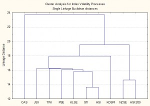
The research confirms the presence of a number of typical characteristics of volatility processes for emerging markets that have previously been identified in empirical research conducted in developed markets.  These characteristics include volatility clustering, long memory, and asymmetry.   There appears to be strong evidence of a region-wide regime shift in volatility processes during the Asian crises in 1997, and a less prevalent regime shift in September 2001. We find evidence from multivariate analysis that the sample separates into two distinct groups:  a lower volatility group comprising the Australian and New Zealand indices and a higher volatility group comprising the majority of the other indices.

SSALGOTRADING AD

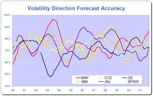
Models developed within the single- and two-factor REGARCH framework of Alizadeh, Brandt and Diebold (2002) provide a good fit for many of the volatility series and in many cases have performance characteristics that compare favorably with other classes of models with high R-squares, low MAPE and direction prediction accuracy of 70% or more.   On the debit side, many of the models demonstrate considerable variation in explanatory power over time, often associated with regime shifts or major market events, and this is typically accompanied by some model parameter drift and/or instability.

Single equation ARFIMA-GARCH models appear to be a robust and reliable framework for modeling asset volatility processes, as they are capable of capturing both the short- and long-memory effects in the volatility processes, as well as GARCH effects in the kurtosis process.   The available procedures for estimating the degree of fractional integration in the volatility processes produce estimates that appear to vary widely for processes which include both short- and long- memory effects, but the overall conclusion is that long memory effects are at least as important as they are for volatility processes in developed markets.  Simple extensions to the single-equation models, which include regressor lags of related volatility series, add significant explanatory power to the models and suggest the existence of Granger-causality relationships between processes.

Extending the modeling procedures into the realm of models which incorporate systems of equations provides evidence of two-way Granger causality between certain of the volatility processes and suggests that are fractionally cointegrated, a finding shared with parallel studies of volatility processes in developed markets.

Download paper here.

Resources for Quantitative Analysts

Two of the smartest econometricians I know are Prof. Stephen Taylor of Lancaster University, and Prof. James Davidson of Exeter University.

I recall spending many profitable hours in the 1980’s with Stephen’s book Modelling Financial Time Series, which I am pleased to see has now been reprinted in a second edition.  For a long time this was the best available book on the topic and it remains a classic. It has been surpassed by very few books, one being Stephen’s later work Asset Price Dynamics, Volatility and Prediction.  This is a superb exposition, one that will repay close study.

James Davidson is one of the smartest minds in econometrics. Not only is his research of the highest caliber, he has somehow managed (in his spare time!) to develop one of the most advanced econometrics packages available.  Based on Jurgen Doornik’s Ox programming system, the Time Series Modelling package covers almost every conceivable model type, including regression models, ARIMA, ARFIMA and other single equation models, systems of equations, panel data models, GARCH and other heteroscedastic models and regime switching models, accompanied by very comprehensive statistical testing capabilities.  Furthermore, TSM is very well documented and despite being arguably the most advanced system of its kind it is inexpensive relative to alternatives.  James’s research output is voluminous and often highly complex.  His book, Econometric Theory, is an excellent guide to the state of the art, but not for the novice (or the faint hearted!).

Those looking for a kinder, gentler introduction to econometrics would do well to acquire a copy of Prof. Chris Brooks’s Introductory Econometrics for Finance. This covers most of the key ideas, from regression, through ARMA, GARCH, panel data models, cointegration, regime switching and volatility modeling.  Not only is the coverage comprehensive, Chris’s explanation of the concepts is delightfully clear and illustrated with interesting case studies which he analyzes using the EViews econometrics package.    Although not as advanced as TSM, EViews has everything that most quantitative analysts are likely to require in a modeling system and is very well suited to Chris’s teaching style.  Chris’s research output is enormous and covers a great many topics of interest to financial market analysts, in the same lucid style.

Can Machine Learning Techniques Be Used To Predict Market Direction? The 1,000,000 Model Test.

During the 1990’s the advent of Neural Networks unleashed a torrent of research on their applications in financial markets, accompanied by some rather extravagant claims about their predicative abilities.  Sadly, much of the research proved to be sub-standard and the results illusionary, following which the topic was largely relegated to the bleachers, at least in the field of financial market research.

With the advent of new machine learning techniques such as Random Forests, Support Vector Machines and Nearest Neighbor Classification, there has been a resurgence of interest in non-linear modeling techniques and a flood of new research, a fair amount of it supportive of their potential for forecasting financial markets.  Once again, however, doubts about the quality of some of the research bring the results into question.

SSALGOTRADING AD

Against this background I and my co-researcher Dan Rico set out to address the question of whether these new techniques really do have predicative power, more specifically the ability to forecast market direction.  Using some excellent MatLab toolboxes and a new software package, an Excel Addin called 11Ants, that makes large scale testing of multiple models a snap, we examined over 1,000,000 models and model-ensembles, covering just about every available non-linear technique.  The data set for our study comprised daily prices for a selection of US equity securities, together with a large selection of technical indicators for which some other researchers have claimed explanatory power.

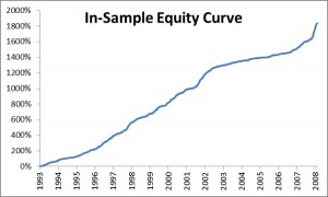
In-Sample Equity Curve for Best Performing Nonlinear Model

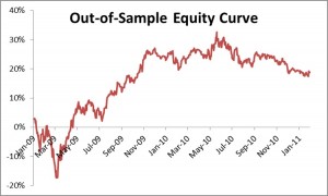
The answer provided by our research was, without exception, in the negative: not one of the models tested showed any significant ability to predict the direction of any of the securities in our data set.  Furthermore, our study found that the best-performing models favored raw price data over technical indicator variables, suggesting that the latter have little explanatory power.

As with Neural Networks, the principal difficulty with non-linear techniques appears to be curve-fitting and a failure to generalize:  while it is very easy to find models that provide an excellent fit to in-sample data, the forecasting performance out-of-sample is often very poor.

Out-of-Sample Equity Curve for Best Performing Nonlinear Model

Some caveats about our own research apply.  First and foremost, it is of course impossible to prove a hypothesis in the negative.  Secondly, it is plausible that some markets are less efficient than others:  some studies have claimed success in developing predictive models due to the (relative) inefficiency of the F/X and futures markets, for example.  Thirdly, the choice of sample period may be criticized:  it could be that the models were over-conditioned on a too- lengthy in-sample data set, which in one case ran from 1993 to 2008, with just two years (2009-2010) of out-of-sample data.  The choice of sample was deliberate, however:  had we omitted the 2008 period from the “learning” data set, it would be very easy to criticize the study for failing to allow the algorithms to learn about the exceptional behavior of the markets during that turbulent year.

Despite these limitations, our research casts doubt on the findings of some less-extensive studies, that may be the result of sample-selection bias.  One characteristic of the most credible studies finding evidence in favor of market predictability, such as those by Pesaran and Timmermann, for instance (see paper for citations), is that the models they employ tend to incorporate independent explanatory variables, such as yield spreads, which do appear to have real explanatory power.  The finding of our study suggest that, absent such explanatory factors, the ability to predict markets using sophisticated non-linear techniques applied to price data alone may prove to be as illusionary as it was in the 1990’s.


ONE MILLION MODELS

Range-Based EGARCH Option Pricing Models (REGARCH)

The research in this post and the related paper on Range Based EGARCH Option pricing Models is focused on the innovative range-based volatility models introduced in Alizadeh, Brandt, and Diebold (2002) (hereafter ABD).  We develop new option pricing models using multi-factor diffusion approximations couched within this theoretical framework and examine their properties in comparison with the traditional Black-Scholes model.

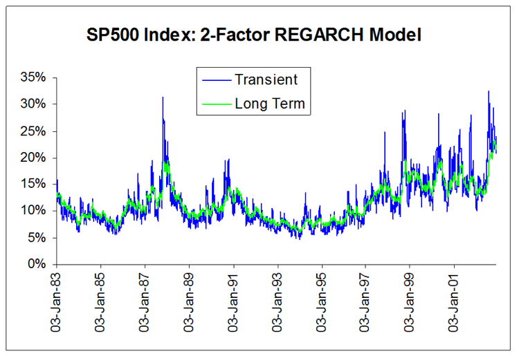
The two-factor version of the model, which I have applied successfully in various option arbitrage strategies, encapsulates the intuively appealing idea of a trending long term mean volatility process, around which oscillates a mean-reverting, transient volatility process.  The option pricing model also incorporates asymmetry/leverage effects and well as correlation effects between the asset return and volatility processes, which results in a volatility skew.

The core concept behind Range-Based Exponential GARCH model is Log-Range estimator discussed in an earlier post on volatility metrics, which contains a lengthy exposition of various volatility estimators and their properties. (Incidentally, for those of you who requested a copy of my paper on Estimating Historical Volatility, I have updated the post to include a link to the pdf).

SSALGOTRADING AD

We assume that the log stock price s follows a drift-less Brownian motion ds = sdW. The volatility of daily log returns, denoted h= s/sqrt(252), is assumed constant within each day, at ht from the beginning to the end of day t, but is allowed to change from one day to the next, from ht at the end of day t to ht+1 at the beginning of day t+1.  Under these assumptions, ABD show that the log range, defined as:

is to a very good approximation distributed as

where N[m; v] denotes a Gaussian distribution with mean m and variance v. The above equation demonstrates that the log range is a noisy linear proxy of log volatility ln ht.  By contrast, according to the results of Alizadeh, Brandt,and Diebold (2002), the log absolute return has a mean of 0.64 + ln ht and a variance of 1.11. However, the distribution of the log absolute return is far from Gaussian.  The fact that both the log range and the log absolute return are linear log volatility proxies (with the same loading of one), but that the standard deviation of the log range is about one-quarter of the standard deviation of the log absolute return, makes clear that the range is a much more informative volatility proxy. It also makes sense of the finding of Andersen and Bollerslev (1998) that the daily range has approximately the same informational content as sampling intra-daily returns every four hours.

Except for the model of Chou (2001), GARCH-type volatility models rely on squared or absolute returns (which have the same information content) to capture variation in the conditional volatility ht. Since the range is a more informative volatility proxy, it makes sense to consider range-based GARCH models, in which the range is used in place of squared or absolute returns to capture variation in the conditional volatility. This is particularly true for the EGARCH framework of Nelson (1990), which describes the dynamics of log volatility (of which the log range is a linear proxy).

ABD consider variants of the EGARCH framework introduced by Nelson (1990). In general, an EGARCH(1,1) model performs comparably to the GARCH(1,1) model of Bollerslev (1987).  However, for stock indices the in-sample evidence reported by Hentschel (1995) and the forecasting performance presented by Pagan and Schwert (1990) show a slight superiority of the EGARCH specification. One reason for this superiority is that EGARCH models can accommodate asymmetric volatility (often called the “leverage effect,” which refers to one of the explanations of asymmetric volatility), where increases in volatility are associated more often with large negative returns than with equally large positive returns.

The one-factor range-based model (REGARCH 1)  takes the form:

where the returns process Rt is conditionally Gaussian: Rt ~ N[0, ht2]

and the process innovation is defined as the standardized deviation of the log range from its expected value:

Following Engle and Lee (1999), ABD also consider multi-factor volatility models.  In particular, for a two-factor range-based EGARCH model (REGARCH2), the conditional volatility dynamics) are as follows:

and

where ln qt can be interpreted as a slowly-moving stochastic mean around which log volatility  ln ht makes large but transient deviations (with a process determined by the parameters kh, fh and dh).

The parameters q, kq, fq and dq determine the long-run mean, sensitivity of the long run mean to lagged absolute returns, and the asymmetry of absolute return sensitivity respectively.

The intuition is that when the lagged absolute return is large (small) relative to the lagged level of volatility, volatility is likely to have experienced a positive (negative) innovation. Unfortunately, as we explained above, the absolute return is a rather noisy proxy of volatility, suggesting that a substantial part of the volatility variation in GARCH-type models is driven by proxy noise as opposed to true information about volatility. In other words, the noise in the volatility proxy introduces noise in the implied volatility process. In a volatility forecasting context, this noise in the implied volatility process deteriorates the quality of the forecasts through less precise parameter estimates and, more importantly, through less precise estimates of the current level of volatility to which the forecasts are anchored.

read more

2-Factor REGARCH Model for the S&P500 Index

On Testing Direction Prediction Accuracy


As regards the question of forecasting accuracy discussed in the paper on Forecasting Volatility in the S&P 500 Index, there are two possible misunderstandings here that need to be cleared up.  These arise from remarks by one commentator  as follows:

“An above 50% vol direction forecast looks good,.. but “direction” is biased when working with highly skewed distributions!   ..so it would be nice if you could benchmark it against a simple naive predictors to get a feel for significance, -or- benchmark it with a trading strategy and see how the risk/return performs.”

(i) The first point is simple, but needs saying: the phrase “skewed distributions” in the context of volatility modeling could easily be misconstrued as referring to the volatility skew. This, of course, is used to describe to the higher implied vols seen in the Black-Scholes prices of OTM options. But in the Black-Scholes framework volatility is constant, not stochastic, and the “skew” referred to arises in the distribution of the asset return process, which has heavier tails than the Normal distribution (excess Kurtosis and/or skewness). I realize that this is probably not what the commentator meant, but nonetheless it’s worth heading that possible misunderstanding off at the pass, before we go on.

SSALGOTRADING AD

(ii) I assume that the commentator was referring to the skewness in the volatility process, which is characterized by the LogNormal distribution. But the forecasting tests referenced in the paper are tests of the ability of the model to predict the direction of volatility, i.e. the sign of the change in the level of volatility from the current period to the next period. Thus we are looking at, not a LogNormal distribution, but the difference in two LogNormal distributions with equal mean – and this, of course, has an expectation of zero. In other words, the expected level of volatility for the next period is the same as the current period and the expected change in the level of volatility is zero. You can test this very easily for yourself by generating a large number of observations from a LogNormal process, taking the difference and counting the number of positive and negative changes in the level of volatility from one period to the next. You will find, on average, half the time the change of direction is positive and half the time it is negative.

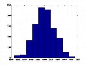
For instance, the following chart shows the distribution of the number of positive changes in the level of a LogNormally distributed random variable with mean and standard deviation of 0.5, for a sample of 1,000 simulations, each of 10,000 observations.  The sample mean (5,000.4) is very close to the expected value of 5,000.

Distribution Number of Positive Direction Changes

So, a naive predictor will forecast volatility to remain unchanged for the next period and by random chance approximately half the time volatility will turn out to be higher and half the time it will turn out to be lower than in the current period. Hence the default probability estimate for a positive change of direction is 50% and you would expect to be right approximately half of the time. In other words, the direction prediction accuracy of the naive predictor is 50%. This, then, is one of the key benchmarks you use to assess the ability of the model to predict market direction. That is what test statistics like Theil’s-U does – measures the performance relative to the naive predictor. The other benchmark we use is the change of direction predicted by the implied volatility of ATM options.
In this context, the model’s 61% or higher direction prediction accuracy is very significant (at the 4% level in fact) and this is reflected in the Theil’s-U statistic of 0.82 (lower is better). By contrast, Theil’s-U for the Implied Volatility forecast is 1.46, meaning that IV is a much worse predictor of 1-period-ahead changes in volatility than the naive predictor.

On its face, it is because of this exceptional direction prediction accuracy that a simple strategy is able to generate what appear to be abnormal returns using the change of direction forecasts generated by the model, as described in the paper. In fact, the situation is more complicated than that, once you introduce the concept of a market price of volatility risk.


Long Memory and Regime Shifts in Asset Volatility

This post covers quite a wide range of concepts in volatility modeling relating to long memory and regime shifts and is based on an article that was published in Wilmott magazine and republished in The Best of Wilmott Vol 1 in 2005.  A copy of the article can be downloaded here.

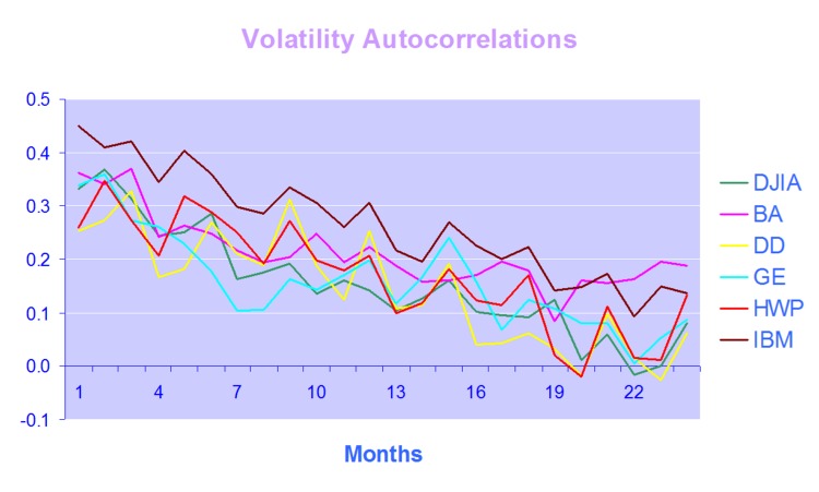
One of the defining characteristics of volatility processes in general (not just financial assets) is the tendency for the serial autocorrelations to decline very slowly.  This effect is illustrated quite clearly in the chart below, which maps the autocorrelations in the volatility processes of several financial assets.

Thus we can say that events in the volatility process for IBM, for instance, continue to exert influence on the process almost two years later.

This feature in one that is typical of a black noise process – not some kind of rap music variant, but rather:

“a process with a 1/fβ spectrum, where β > 2 (Manfred Schroeder, “Fractalschaos, power laws“). Used in modeling various environmental processes. Is said to be a characteristic of “natural and unnatural catastrophes like floods, droughts, bear markets, and various outrageous outages, such as those of electrical power.” Further, “because of their black spectra, such disasters often come in clusters.”” [Wikipedia].

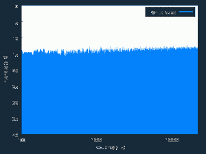
Because of these autocorrelations, black noise processes tend to reinforce or trend, and hence (to some degree) may be forecastable.  This contrasts with a white noise process, such as an asset return process, which has a uniform power spectrum, insignificant serial autocorrelations and no discernable trending behavior:

White Noise Power Spectrum

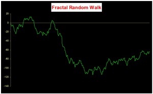
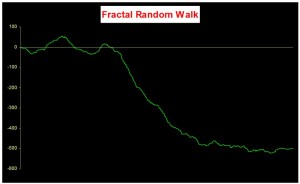
An econometrician might describe this situation by saying that a  black noise process is fractionally integrated order d, where d = H/2, H being the Hurst Exponent.  A way to appreciate the difference in the behavior of a black noise process vs. a white process is by comparing two fractionally integrated random walks generated using the same set of quasi random numbers by Feder’s (1988) algorithm (see p 32 of the presentation on Modeling Asset Volatility).

Fractal Random Walk - White Noise
Fractal Random Walk – White Noise
Fractal Random Walk - Black Noise Process
Fractal Random Walk – Black Noise Process

As you can see. both random walks follow a similar pattern, but the black noise random walk is much smoother, and the downward trend is more clearly discernible.  You can play around with the Feder algorithm, which is coded in the accompanying Excel Workbook on Volatility and Nonlinear Dynamics .  Changing the Hurst Exponent parameter H in the worksheet will rerun the algorithm and illustrate a fractal random walk for a black noise (H > 0.5), white noise (H=0.5) and mean-reverting, pink noise (H<0.5) process.

One way of modeling the kind of behavior demonstrated by volatility process is by using long memory models such as ARFIMA and FIGARCH (see pp 47-62 of the Modeling Asset Volatility presentation for a discussion and comparison of various long memory models).  The article reviews research into long memory behavior and various techniques for estimating long memory models and the coefficient of fractional integration d for a process.

SSALGOTRADING AD

But long memory is not the only possible cause of long term serial correlation.  The same effect can result from structural breaks in the process, which can produce spurious autocorrelations.  The article goes on to review some of the statistical procedures that have been developed to detect regime shifts, due to Bai (1997), Bai and Perron (1998) and the Iterative Cumulative Sums of Squares methodology due to Aggarwal, Inclan and Leal (1999).  The article illustrates how the ICSS technique accurately identifies two changes of regimes in a synthetic GBM process.

In general, I have found the ICSS test to be a simple and highly informative means of gaining insight about a process representing an individual asset, or indeed an entire market.  For example, ICSS detects regime shifts in the process for IBM around 1984 (the time of the introduction of the IBM PC), the automotive industry in the early 1980’s (Chrysler bailout), the banking sector in the late 1980’s (Latin American debt crisis), Asian sector indices in Q3 1997, the S&P 500 index in April 2000 and just about every market imaginable during the 2008 credit crisis.  By splitting a series into pre- and post-regime shift sub-series and examining each segment for long memory effects, one can determine the cause of autocorrelations in the process.  In some cases, Asian equity indices being one example, long memory effects disappear from the series, indicating that spurious autocorrelations were induced by a major regime shift during the 1997 Asian crisis. In most cases, however, long memory effects persist.

Excel Workbook on Volatility and Nonlinear Dynamics 

There are several other topics from chaos theory and nonlinear dynamics covered in the workbook, including:

More on these issues in due course.

Modeling Asset Volatility

I am planning a series of posts on the subject of asset volatility and option pricing and thought I would begin with a survey of some of the central ideas. The attached presentation on Modeling Asset Volatility sets out the foundation for a number of key concepts and the basis for the research to follow.

Perhaps the most important feature of volatility is that it is stochastic rather than constant, as envisioned in the Black Scholes framework.  The presentation addresses this issue by identifying some of the chief stylized facts about volatility processes and how they can be modelled.  Certain characteristics of volatility are well known to most analysts, such as, for instance, its tendency to “cluster” in periods of higher and lower volatility.  However, there are many other typical features that are less often rehearsed and these too are examined in the presentation.

Long Memory
For example, while it is true that GARCH models do a fine job of modeling the clustering effect  they typically fail to capture one of the most important features of volatility processes – long term serial autocorrelation.  In the typical GARCH model autocorrelations die away approximately exponentially, and historical events are seen to have little influence on the behaviour of the process very far into the future.  In volatility processes that is typically not the case, however:  autocorrelations die away very slowly and historical events may continue to affect the process many weeks, months or even years ahead.

Volatility Direction Prediction Accuracy

There are two immediate and very important consequences of this feature.  The first is that volatility processes will tend to trend over long periods – a characteristic of Black Noise or Fractionally Integrated processes, compared to the White Noise behavior that typically characterizes asset return processes.  Secondly, and again in contrast with asset return processes, volatility processes are inherently predictable, being conditioned to a significant degree on past behavior.  The presentation considers the fractional integration frameworks as a basis for modeling and forecasting volatility.

Mean Reversion vs. Momentum
A puzzling feature of much of the literature on volatility is that it tends to stress the mean-reverting behavior of volatility processes.  This appears to contradict the finding that volatility behaves as a reinforcing process, whose long-term serial autocorrelations create a tendency to trend.  This leads to one of the most important findings about asset processes in general, and volatility process in particular: i.e. that the assets processes are simultaneously trending and mean-reverting.  One way to understand this is to think of volatility, not as a single process, but as the superposition of two processes:  a long term process in the mean, which tends to reinforce and trend, around which there operates a second, transient process that has a tendency to produce short term spikes in volatility that decay very quickly.  In other words, a transient, mean reverting processes inter-linked with a momentum process in the mean.  The presentation discusses two-factor modeling concepts along these lines, and about which I will have more to say later.

SSALGOTRADING AD

Cointegration
One of the most striking developments in econometrics over the last thirty years, cointegration is now a principal weapon of choice routinely used by quantitative analysts to address research issues ranging from statistical arbitrage to portfolio construction and asset allocation.  Back in the late 1990’s I and a handful of other researchers realized that volatility processes exhibited very powerful cointegration tendencies that could be harnessed to create long-short volatility strategies, mirroring the approach much beloved by equity hedge fund managers.  In fact, this modeling technique provided the basis for the Caissa Capital volatility fund, which I founded in 2002.  The presentation examines characteristics of multivariate volatility processes and some of the ideas that have been proposed to model them, such as FIGARCH (fractionally-integrated GARCH).

Dispersion Dynamics
Finally, one topic that is not considered in the presentation, but on which I have spent much research effort in recent years, is the behavior of cross-sectional volatility processes, which I like to term dispersion.  It turns out that, like its univariate cousin, dispersion displays certain characteristics that in principle make it highly forecastable.  Given an appropriate model of dispersion dynamics, the question then becomes how to monetize efficiently the insight that such a model offers.  Again, I will have much more to say on this subject, in future.

Market Timing in the S&P 500 Index Using Volatility Forecasts

There has been a good deal of interest in the market timing ideas discussed in my earlier blog post Using Volatility to Predict Market Direction, which discusses the research of Diebold and Christoffersen into the sign predictability induced by volatility dynamics.  The ideas are thoroughly explored in a QuantNotes article from 2006, which you can download here.

There is a follow-up article from 2006 in which Christoffersen, Diebold, Mariano and Tay develop the ideas further to consider the impact of higher moments of the asset return distribution on sign predictability and the potential for market timing in international markets (download here).

Trading Strategy
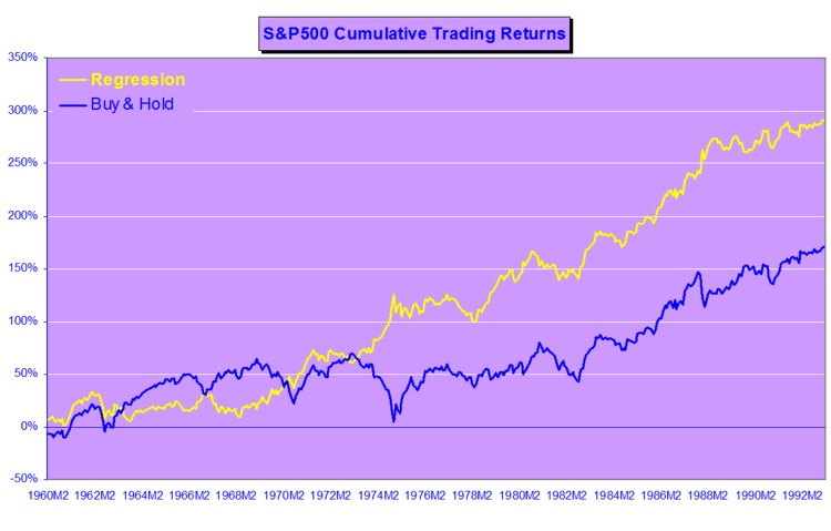
To illustrate some of the possibilities of this approach, we constructed a simple market timing strategy in which a position was taken in the S&P 500 index or in 90-Day T-Bills, depending on an ex-ante forecast of positive returns from the logit regression model (and using an expanding window to estimate the drift coefficient).  We assume that the position is held for 30 days and rebalanced at the end of each period.  In this test we make no allowance for market impact, or transaction costs.

Results
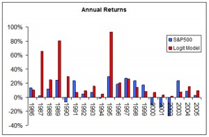
Annual returns for the strategy and for the benchmark S&P 500 Index are shown in the figure below.  The strategy performs exceptionally well in 1987, 1989 and 1995, when the ratio between expected returns and volatility remains close to optimum levels and the direction of the S&P 500 Index is highly predictable,  Of equal interest is that the strategy largely avoids the market downturn of 2000-2002 altogether, a period in which sign probabilities were exceptionally low.

SSALGOTRADING AD

In terms of overall performance, the model enters the market in 113 out of a total of 241 months (47%) and is profitable in 78 of them (69%).  The average gain is 7.5% vs. an average loss of –4.11% (ratio 1.83).  The compound annual return is 22.63%, with an annual volatility of 17.68%, alpha of 14.9% and Sharpe ratio of 1.10.

The under-performance of the strategy in 2003 is explained by the fact that direction-of-change probabilities were rising from a very low base in Q4 2002 and do not reach trigger levels until the end of the year.  Even though the strategy out-performed the Index by a substantial margin of 6% , the performance in 2005 is of concern as market volatility was very low and probabilities overall were on a par with those seen in 1995.  Further tests are required to determine whether the failure of the strategy to produce an exceptional performance on par with 1995 was the result of normal statistical variation or due to changes in the underlying structure of the process requiring model recalibration.

Future Research & Development
The obvious next step is to develop the approach described above to formulate trading strategies based on sign forecasting in a universe of several assets, possibly trading binary options.  The approach also has potential for asset allocation, portfolio theory and risk management applications.

Market Timing in the S&amp;P500 Index
Market Timing in the S&P500 Index

Robustness in Quantitative Research and Trading

What is Strategy Robustness?  What is its relevance to Quantitative Research and Trading?

One of the most highly desired properties of any financial model or investment strategy, by investors and managers alike, is robustness.  I would define robustness as the ability of the strategy to deliver a consistent  results across a wide range of market conditions.  It, of course, by no means the only desirable property – investing in Treasury bills is also a pretty robust strategy, although the returns are unlikely to set an investor’s pulse racing – but it does ensure that the investor, or manager, is unlikely to be on the receiving end of an ugly surprise when market conditions adjust.

Robustness is not the same thing as low volatility, which also tends to be a characteristic highly prized by many investors.  A strategy may operate consistently, with low volatility in certain market conditions, but behave very differently in other.  For instance, a delta-hedged short-volatility book containing exotic derivative positions.   The point is that empirical researchers do not know the true data-generating process for the markets they are modeling. When specifying an empirical model they need to make arbitrary assumptions. An example is the common assumption that assets returns follow a Gaussian distribution.  In fact, the empirical distribution of the great majority of asset process exhibit the characteristic of “fat tails”, which can result from the interplay between multiple market states with random transitions.  See this post for details:

http://jonathankinlay.com/2014/05/a-quantitative-analysis-of-stationarity-and-fat-tails/


In statistical arbitrage, for example, quantitative researchers often make use of cointegration models to build pairs trading strategies.  However the testing procedures used in current practice are not sufficient powerful to distinguish between cointegrated processes and those whose evolution just happens to correlate temporarily, resulting in the frequent breakdown in cointegrating relationships.  For instance, see this post:

http://jonathankinlay.com/2017/06/statistical-arbitrage-breaks/

Modeling Assumptions are Often Wrong – and We Know It

We are, of course, not the first to suggest that empirical models are misspecified:

“All models are wrong, but some are useful” (Box 1976, Box and Draper 1987).


Martin Feldstein (1982: 829): “In practice all econometric specifications are necessarily false models.”


Luke Keele (2008: 1): “Statistical models are always simplifications, and even the most complicated model will be a pale imitation of reality.”


Peter Kennedy (2008: 71): “It is now generally acknowledged that econometric models are false and there is no hope, or pretense, that through them truth will be found.”

During the crash of 2008 quantitative Analysts and risk managers found out the hard way that the assumptions underpinning the copula models used to price and hedge credit derivative products were highly sensitive to market conditions.  In other words, they were not robust.  See this post for more on the application of copula theory in risk management:

http://jonathankinlay.com/2017/01/copulas-risk-management/


Robustness Testing in Quantitative Research and Trading

We interpret model misspecification as model uncertainty. Robustness tests analyze model uncertainty by comparing a baseline model to plausible alternative model specifications.  Rather than trying to specify models correctly (an impossible task given causal complexity), researchers should test whether the results obtained by their baseline model, which is their best attempt of optimizing the specification of their empirical model, hold when they systematically replace the baseline model specification with plausible alternatives. This is the practice of robustness testing.

SSALGOTRADING AD

Robustness testing analyzes the uncertainty of models and tests whether estimated effects of interest are sensitive to changes in model specifications. The uncertainty about the baseline model’s estimated effect size shrinks if the robustness test model finds the same or similar point estimate with smaller standard errors, though with multiple robustness tests the uncertainty likely increases. The uncertainty about the baseline model’s estimated effect size increases of the robustness test model obtains different point estimates and/or gets larger standard errors. Either way, robustness tests can increase the validity of inferences.

Robustness testing replaces the scientific crowd by a systematic evaluation of model alternatives.

Robustness in Quantitative Research

In the literature, robustness has been defined in different ways:

  • as same sign and significance (Leamer)
  • as weighted average effect (Bayesian and Frequentist Model Averaging)
  • as effect stability We define robustness as effect stability.

Parameter Stability and Properties of Robustness

Robustness is the share of the probability density distribution of the baseline model that falls within the 95-percent confidence interval of the baseline model.  In formulaeic terms:

Formula

  • Robustness is left-–right symmetric: identical positive and negative deviations of the robustness test compared to the baseline model give the same degree of robustness.
  • If the standard error of the robustness test is smaller than the one from the baseline model, ρ converges to 1 as long as the difference in point estimates is negligible.
  • For any given standard error of the robustness test, ρ is always and unambiguously smaller the larger the difference in point estimates.
  • Differences in point estimates have a strong influence on ρ if the standard error of the robustness test is small but a small influence if the standard errors are large.

Robustness Testing in Four Steps

  1. Define the subjectively optimal specification for the data-generating process at hand. Call this model the baseline model.
  2. Identify assumptions made in the specification of the baseline model which are potentially arbitrary and that could be replaced with alternative plausible assumptions.
  3. Develop models that change one of the baseline model’s assumptions at a time. These alternatives are called robustness test models.
  4. Compare the estimated effects of each robustness test model to the baseline model and compute the estimated degree of robustness.

Model Variation Tests

Model variation tests change one or sometimes more model specification assumptions and replace with an alternative assumption, such as:

  • change in set of regressors
  • change in functional form
  • change in operationalization
  • change in sample (adding or subtracting cases)

Example: Functional Form Test

The functional form test examines the baseline model’s functional form assumption against a higher-order polynomial model. The two models should be nested to allow identical functional forms. As an example, we analyze the ‘environmental Kuznets curve’ prediction, which suggests the existence of an inverse u-shaped relation between per capita income and emissions.
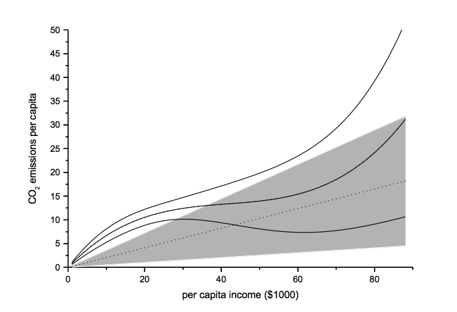
Emissions and percapitaincome

Note: grey-shaded area represents confidence interval of baseline model

Another example of functional form testing is given in this review of Yield Curve Models:

http://jonathankinlay.com/2018/08/modeling-the-yield-curve/

Random Permutation Tests

Random permutation tests change specification assumptions repeatedly. Usually, researchers specify a model space and randomly and repeatedly select model from this model space. Examples:

  • sensitivity tests (Leamer 1978)
  • artificial measurement error (Plümper and Neumayer 2009)
  • sample split – attribute aggregation (Traunmüller and Plümper 2017)
  • multiple imputation (King et al. 2001)

We use Monte Carlo simulation to test the sensitivity of the performance of our Quantitative Equity strategy to changes in the price generation process and also in model parameters:

http://jonathankinlay.com/2017/04/new-longshort-equity/

Structured Permutation Tests

Structured permutation tests change a model assumption within a model space in a systematic way. Changes in the assumption are based on a rule, rather than random.  Possibilities here include:

  • sensitivity tests (Levine and Renelt)
  • jackknife test
  • partial demeaning test

Example: Jackknife Robustness Test

The jackknife robustness test is a structured permutation test that systematically excludes one or more observations from the estimation at a time until all observations have been excluded once. With a ‘group-wise jackknife’ robustness test, researchers systematically drop a set of cases that group together by satisfying a certain criterion – for example, countries within a certain per capita income range or all countries on a certain continent. In the example, we analyse the effect of earthquake propensity on quake mortality for countries with democratic governments, excluding one country at a time. We display the results using per capita income as information on the x-axes.
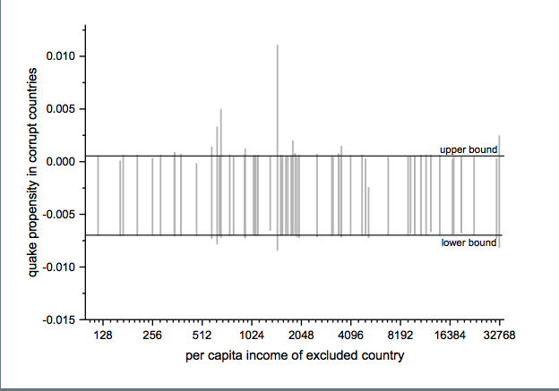
jackknife

Upper and lower bound mark the confidence interval of the baseline model.

Robustness Limit Tests

Robustness limit tests provide a way of analyzing structured permutation tests. These tests ask how much a model specification has to change to render the effect of interest non-robust. Some examples of robustness limit testing approaches:

  • unobserved omitted variables (Rosenbaum 1991)
  • measurement error
  • under- and overrepresentation
  • omitted variable correlation

For an example of limit testing, see this post on a review of the Lognormal Mixture Model:

http://jonathankinlay.com/2018/08/the-lognormal-mixture-variance-model/

Summary on Robustness Testing

Robustness tests have become an integral part of research methodology. Robustness tests allow to study the influence of arbitrary specification assumptions on estimates. They can identify uncertainties that otherwise slip the attention of empirical researchers. Robustness tests offer the currently most promising answer to model uncertainty.
Forecasting Volatility in the S&P500 Index

Several people have asked me for copies of this research article, which develops a new theoretical framework, the ARFIMA-GARCH model as a basis for forecasting volatility in the S&P 500 Index.  I am in the process of updating the research, but in the meantime a copy of the original paper is available here

In this analysis we are concerned with the issue of whether market forecasts of volatility, as expressed in the Black-Scholes implied volatilities of at-the-money European options on the S&P500 Index, are superior to those produced by a new forecasting model in the GARCH framework which incorporates long-memory effects.  The ARFIMA-GARCH model, which uses high frequency data comprising 5-minute returns, makes volatility the subject process of interest, to which innovations are introduced via a volatility-of-volatility (kurtosis) process.  Despite performing robustly in- and out-of-sample, an encompassing regression indicates that the model is unable to add to the information already contained in market forecasts.  However, unlike model forecasts, implied volatility forecasts show evidence of a consistent and substantial bias.  Furthermore, the model is able to correctly predict the direction of volatility approximately 62% of the time whereas market forecasts have very poor direction prediction ability.  This suggests that either option markets may be inefficient, or that the option pricing model is mis-specified.  To examine this hypothesis, an empirical test is carried out in which at-the-money straddles are bought or sold (and delta-hedged) depending on whether the model forecasts exceed or fall below implied volatility forecasts.  This simple strategy generates an annual compound return of 18.64% over a four year out-of-sample period, during which the annual return on the S&P index itself was -7.24%.  Our findings suggest that, over the period of analysis, investors required an additional risk premium of 88 basis points of incremental return for each unit of volatility risk.