
This post covers quite a wide range of concepts in volatility modeling relating to long memory and regime shifts and is based on an article that was published in Wilmott magazine and republished in The Best of Wilmott Vol 1 in 2005. A copy of the article can be downloaded here.
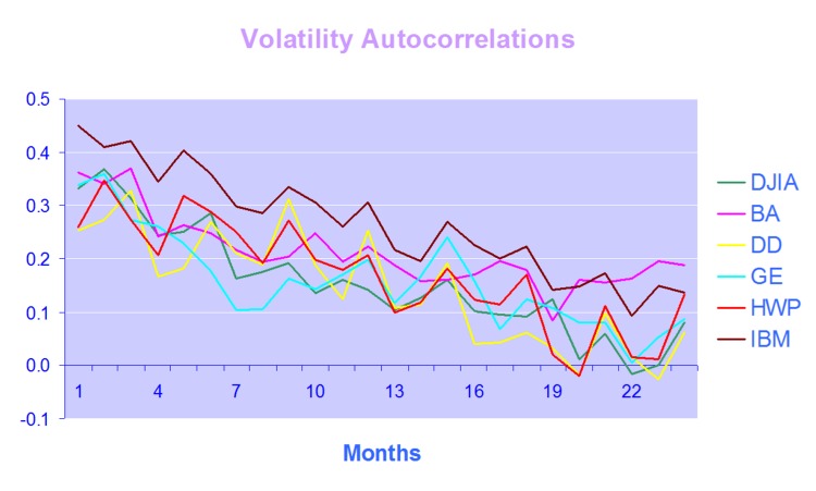
One of the defining characteristics of volatility processes in general (not just financial assets) is the tendency for the serial autocorrelations to decline very slowly. This effect is illustrated quite clearly in the chart below, which maps the autocorrelations in the volatility processes of several financial assets.
Thus we can say that events in the volatility process for IBM, for instance, continue to exert influence on the process almost two years later.
This feature in one that is typical of a black noise process – not some kind of rap music variant, but rather:
“a process with a 1/fβ spectrum, where β > 2 (Manfred Schroeder, “Fractals, chaos, power laws“). Used in modeling various environmental processes. Is said to be a characteristic of “natural and unnatural catastrophes like floods, droughts, bear markets, and various outrageous outages, such as those of electrical power.” Further, “because of their black spectra, such disasters often come in clusters.”” [Wikipedia].
Because of these autocorrelations, black noise processes tend to reinforce or trend, and hence (to some degree) may be forecastable. This contrasts with a white noise process, such as an asset return process, which has a uniform power spectrum, insignificant serial autocorrelations and no discernable trending behavior:

An econometrician might describe this situation by saying that a black noise process is fractionally integrated order d, where d = H/2, H being the Hurst Exponent. A way to appreciate the difference in the behavior of a black noise process vs. a white process is by comparing two fractionally integrated random walks generated using the same set of quasi random numbers by Feder’s (1988) algorithm (see p 32 of the presentation on Modeling Asset Volatility).


As you can see. both random walks follow a similar pattern, but the black noise random walk is much smoother, and the downward trend is more clearly discernible. You can play around with the Feder algorithm, which is coded in the accompanying Excel Workbook on Volatility and Nonlinear Dynamics . Changing the Hurst Exponent parameter H in the worksheet will rerun the algorithm and illustrate a fractal random walk for a black noise (H > 0.5), white noise (H=0.5) and mean-reverting, pink noise (H<0.5) process.
One way of modeling the kind of behavior demonstrated by volatility process is by using long memory models such as ARFIMA and FIGARCH (see pp 47-62 of the Modeling Asset Volatility presentation for a discussion and comparison of various long memory models). The article reviews research into long memory behavior and various techniques for estimating long memory models and the coefficient of fractional integration d for a process.

But long memory is not the only possible cause of long term serial correlation. The same effect can result from structural breaks in the process, which can produce spurious autocorrelations. The article goes on to review some of the statistical procedures that have been developed to detect regime shifts, due to Bai (1997), Bai and Perron (1998) and the Iterative Cumulative Sums of Squares methodology due to Aggarwal, Inclan and Leal (1999). The article illustrates how the ICSS technique accurately identifies two changes of regimes in a synthetic GBM process.
In general, I have found the ICSS test to be a simple and highly informative means of gaining insight about a process representing an individual asset, or indeed an entire market. For example, ICSS detects regime shifts in the process for IBM around 1984 (the time of the introduction of the IBM PC), the automotive industry in the early 1980’s (Chrysler bailout), the banking sector in the late 1980’s (Latin American debt crisis), Asian sector indices in Q3 1997, the S&P 500 index in April 2000 and just about every market imaginable during the 2008 credit crisis. By splitting a series into pre- and post-regime shift sub-series and examining each segment for long memory effects, one can determine the cause of autocorrelations in the process. In some cases, Asian equity indices being one example, long memory effects disappear from the series, indicating that spurious autocorrelations were induced by a major regime shift during the 1997 Asian crisis. In most cases, however, long memory effects persist.
Excel Workbook on Volatility and Nonlinear Dynamics
There are several other topics from chaos theory and nonlinear dynamics covered in the workbook, including:
- Generation of the Sierpinski triangle
- Estimation of the Hurst Exponent in various series (Industrial Production, DJIA, S&P500)
- Logistic and Henon attractors
- Estimation of the fractal dimension and correlation integral for the S&P500 index
More on these issues in due course.