Forecasting Market Indices Using Stacked Autoencoders & LSTM

Quality Research vs. Poor Research

The stem paper for this post is:

Bao W, Yue J, Rao Y (2017) A deep learning framework for financial time series using
stacked autoencoders and long-short term memory. PLoS ONE 12(7): e0180944. https://doi.org/10.1371/journal.pone.0180944

The chief claim by the researchers is that 90% to 95% 1-day ahead forecast accuracy can be achieved for a selection of market indices, including the S&P500 and Dow Jones Industrial Average, using a deep learning network of stacked autoencoders and LSTM layers, acting on data transformed using the Haar Discrete Wavelet Transform. The raw data comprises daily data for the index, around a dozen standard technical indicators, the US dollar index and an interest rate series.

Before we go into any detail let’s just step back and look at the larger picture. We have:

  • Unknown researchers
  • A journal from outside the field of finance
  • A paper replete with pretty colored images, but very skimpy detail on the methodology
  • A claimed result that lies far beyond the bounds of credibility

There’s enough red flags here to start a stampede at Pamplona. Let’s go through them one by one:

  1. Everyone is unknown at some point in their career. But that’s precisely why you partner with a widely published author. It gives the reader confidence that the paper isn’t complete garbage.
  2. Not everyone gets to publish in the Journal of Finance. I get that. How many of us were regular readers of the Journal of Political Economy before Black and Scholes published their famous paper on option pricing in 1973? Nevertheless, a finance paper published in a medical journal does not inspire great confidence.
  3. Read almost any paper by a well known researcher and you will find copious detail on the methodology. These days, the paper is often accompanied by a Git repo (add 3 stars for this!). Academics producing quality research want readers to be able to replicate and validate their findings.
    In this paper there are lots of generic, pretty colored graphics of deep learning networks, but no code repo and very little detail on the methodology. If you don’t want to publish details because the methodology is proprietary and potentially valuable, then do what I do: don’t publish at all.
  4. One-day ahead forecasting accuracy of 53%-55% is good (52%-53% in HFT). 60% accuracy is outstanding. 90% – 95% is unbelievable. It’s a license to print money. So what we are being asked to believe is through a combination of data smoothing (which is all DWT is), dimensionality reduction (stacked autoencoders) and long-memory modeling, we can somehow improve forecasting accuracy over, say, a gradient boosted tree baseline, by something like 40%. It simply isn’t credible.

These simple considerations should be enough for any experienced quant to give the paper a wide berth.

Digging into the Methodology

  1. Discrete Wavelet Transform

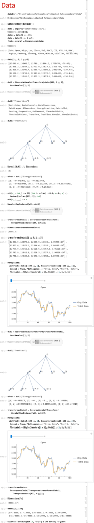
So we start from a raw dataset with variables that closely match those described in the paper (see headers for details). Of course, I don’t know the parameter values they used for most of the technical indicators, but it possibly doesn’t matter all that much.

Note that I am applying DWT using the Haar wavelet twice: once to the original data and then again to the transformed data. This has the effect of filtering out higher frequency “noise” in the data, which is the object of the exercise. If follow this you will also see that the DWT actually adds noisy fluctuations to the US Dollar index and 13-Week TBill series. So these should be excluded from the de-noising process. You can see how the DWT denoising process removes some of the higher frequency fluctuations from the opening price, for instance:

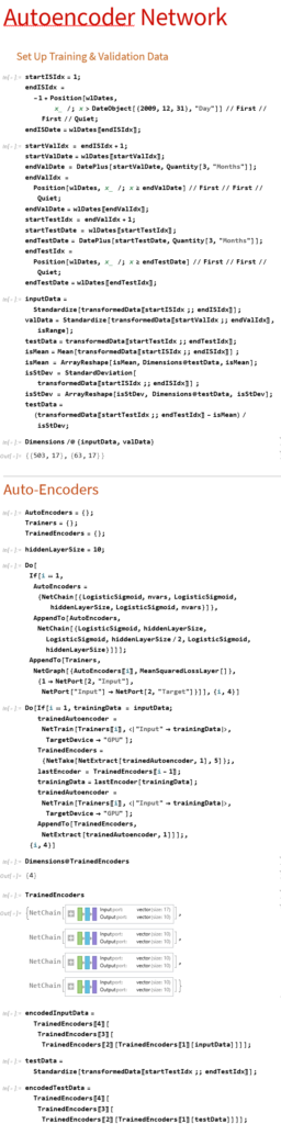
2. Stacked Autoencoders

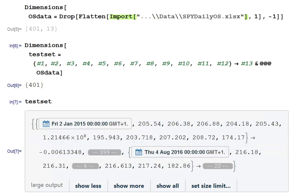
First up, we need to produce data for training, validation and testing. I am doing this for just the first batch of data. We would then move the window forward + 3 months, rinse and repeat.

Note that:

(1) The data is being standardized. If you don’t do this the outputs from the autoencoders is mostly just 1s and 0s. Same happens if you use Min/Max scaling.

(2) We use the mean and standard deviation from the training dataset to normalize the test dataset. This is a trap that too many researchers fall into – standardizing the test dataset using the mean and standard deviation of the test dataset is feeding forward information.

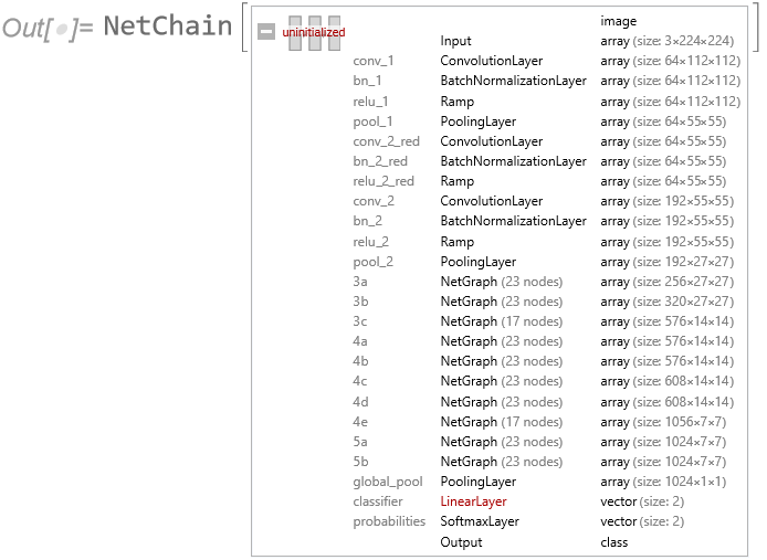
The Autoencoder stack uses a hidden layer of size 10 in each encoder. We strip the output layer from the first encoder and use the hidden layer as inputs to the second autoencoder, and so on:

3. Benchmark Model

Before we plow on any further lets do a sanity check. We’ll use the Predict function to see if we’re able to get any promising-looking results. Here we are building a Gradient Boosted Trees predictor that maps the autoencoded training data to the corresponding closing prices of the index, one step ahead.

Next we use the predictor on the test dataset to produce 1-step-ahead forecasts for the closing price of the index.

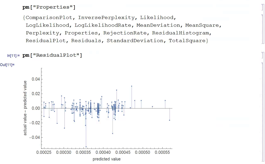
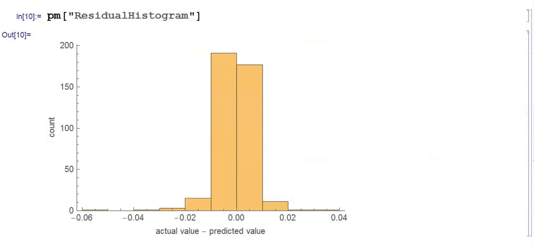
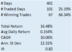
Finally, we construct a trading model, as described in the paper, in which we go long or short the index depending on whether the forecast is above or below the current index level. The results do not look good (see below).

Now, admittedly, an argument can be made that a properly constructed LSTM model would outperform a simple gradient-boosted tree – but not by the amount that would be required to improve the prediction accuracy from around 50% to nearer 95%, the level claimed in the paper. At most I would expect to see a 1% to 5% improvement in forecast accuracy.

So what this suggests to me is that the researchers have got something wrong, by somehow allowing forward information to leak into the modeling process. The most likely culprits are:

  1. Applying DWT transforms to the entire dataset, instead of the training and test sets individually
  2. Standardzing the test dataset using the mean and standard deviation of the test dataset, instead of the training data set

A More Complete Attempt to Replicate the Research

There’s a much more complete attempt at replicating the research in this Git repo

As the repo author writes:

My attempts haven’t been succesful so far. Given the very limited comments regarding implementation in the article, it may be the case that I am missing something important, however the results seem too good to be true, so my assumption is that the authors have a bug in their own implementation. I would of course be happy to be proven wrong about this statement 😉

Conclusion

Over time, as one’s experience as a quant deepens, you learn to recognize the signs of shoddy research and save yourself the effort of trying to replicate it. It’s actually easier these days for researchers to fool themselves (and their readers) that they have uncovered something interesting, because of the facility with which complex algorithms can be deployed in an inappropriate way.

Postscript

 This paper echos my concerns about the incorrect use of wavelets in a forecasting context:

The incorrect development of these wavelet-based forecasting models occurs during wavelet decomposition (the process of extracting high- and low-frequency information into different sub-time series known as wavelet and scaling coefficients, respectively) and as a result introduces error into the forecast model inputs. The source of this error is due to the boundary condition that is associated with wavelet decomposition (and the wavelet and scaling coefficients) and is linked to three main issues: 1) using ‘future data’ (i.e., data from the future that is not available); 2) inappropriately selecting decomposition levels and wavelet filters; and 3) not carefully partitioning calibration and validation data.

Transfer Learning

Building a deep learning neural network is a complicated and time-consuming task. For some problems it can be easier to re-purpose an existing deep learning model, making minor adjustments to a small number of layers to achieve desired architecture.

In his new book Introduction to Machine Learning, Etienne Bernard gives a nice example of the technique.

We begin with a dataset comprising images of two types of mushroom, with the aim of building a specialized image classifier.

Using a Neural Network for Feature Extraction

We start from the Wolfram ImageIdentify net, which is a 24-layer convolutional neural network trained on around 4000 image types.

net=NetModel[“Wolfram ImageIdentify Net V1”]

In its current form the net is too generalized for our task:

Mushroom

So instead of using the net in raw form, we use the first 22 layers as a feature extractor. This will preprocess each image to obtain features that are semantically richer than simple pixel values. We can then train a classifier on top of these new features, producing a logistic regression model:

c=Classify[dsTrain,FeatureExtractor->NetTake[net,22]]

The classifier can now distinguish between different types of mushrooms:

The classifier achieves around 88% accuracy on a test set constructed from a web image search:

dsTest = AssociationMap[
WebImageSearch[#, “Thumbnails”, 10] &, {“Morel”,
“Bolete”}] /. $Failed -> Nothing // Quiet;
ClassifierMeasurements[c, test, “Accuracy”,
ComputeUncertainty -> True]

0.88 +/- 0.09

This is much better than training directly on the underlying pixel values, which would result in an accuracy of around 44%, worse than random guessing.

Neural Network Transfer Learning

Moving on from Etienne’s feature extraction approach, we next try creating a new neural network by re-using the first 22 layers of the ImageIdentify network, adding two new layers (a LinearLayer and SoftmaxLayer) for mushroom classification:

changedNet=Drop[net,-2];
newNet=NetJoin[changedNet,NetChain[Association[“classifier”->LinearLayer[],”probabilities”->SoftmaxLayer[]],”Output”->NetDecoder[{“Class”,{“Bolete”,”Morel”}}]]]

We re-train the new network using the mushroom training dataset, holding the weights for the first 22 layers at their existing values (i.e. only training the last two, new layers):

trainedNet=NetTrain[newNet,Normal@dsTrain,LearningRateMultipliers->{“classifier”->1,_->0},BatchSize->16,TargetDevice->”GPU”]

Next, create a new test dataset and test the new neural network’s accuracy:

dsTest=AssociationMap[WebImageSearch[#,”Thumbnails”,10] &,{“Morel”,”Bolete”}] /. $Failed->Missing[] //Quiet;

The new net achieves 100% accuracy on the test dataset:

trainedNet[DeleteMissing@dsTest[“Bolete”]]

{“Bolete”, “Bolete”, “Bolete”, “Bolete”, “Bolete”, “Bolete”, \
“Bolete”, “Bolete”, “Bolete”}

trainedNet[DeleteMissing@dsTest[“Morel”]]

{“Morel”, “Morel”, “Morel”, “Morel”, “Morel”, “Morel”, “Morel”, \
“Morel”}

Can Machine Learning Techniques Be Used To Predict Market Direction? The 1,000,000 Model Test.

During the 1990’s the advent of Neural Networks unleashed a torrent of research on their applications in financial markets, accompanied by some rather extravagant claims about their predicative abilities.  Sadly, much of the research proved to be sub-standard and the results illusionary, following which the topic was largely relegated to the bleachers, at least in the field of financial market research.

With the advent of new machine learning techniques such as Random Forests, Support Vector Machines and Nearest Neighbor Classification, there has been a resurgence of interest in non-linear modeling techniques and a flood of new research, a fair amount of it supportive of their potential for forecasting financial markets.  Once again, however, doubts about the quality of some of the research bring the results into question.

SSALGOTRADING AD

Against this background I and my co-researcher Dan Rico set out to address the question of whether these new techniques really do have predicative power, more specifically the ability to forecast market direction.  Using some excellent MatLab toolboxes and a new software package, an Excel Addin called 11Ants, that makes large scale testing of multiple models a snap, we examined over 1,000,000 models and model-ensembles, covering just about every available non-linear technique.  The data set for our study comprised daily prices for a selection of US equity securities, together with a large selection of technical indicators for which some other researchers have claimed explanatory power.

In-Sample Equity Curve for Best Performing Nonlinear Model

The answer provided by our research was, without exception, in the negative: not one of the models tested showed any significant ability to predict the direction of any of the securities in our data set.  Furthermore, our study found that the best-performing models favored raw price data over technical indicator variables, suggesting that the latter have little explanatory power.

As with Neural Networks, the principal difficulty with non-linear techniques appears to be curve-fitting and a failure to generalize:  while it is very easy to find models that provide an excellent fit to in-sample data, the forecasting performance out-of-sample is often very poor.

Out-of-Sample Equity Curve for Best Performing Nonlinear Model

Some caveats about our own research apply.  First and foremost, it is of course impossible to prove a hypothesis in the negative.  Secondly, it is plausible that some markets are less efficient than others:  some studies have claimed success in developing predictive models due to the (relative) inefficiency of the F/X and futures markets, for example.  Thirdly, the choice of sample period may be criticized:  it could be that the models were over-conditioned on a too- lengthy in-sample data set, which in one case ran from 1993 to 2008, with just two years (2009-2010) of out-of-sample data.  The choice of sample was deliberate, however:  had we omitted the 2008 period from the “learning” data set, it would be very easy to criticize the study for failing to allow the algorithms to learn about the exceptional behavior of the markets during that turbulent year.

Despite these limitations, our research casts doubt on the findings of some less-extensive studies, that may be the result of sample-selection bias.  One characteristic of the most credible studies finding evidence in favor of market predictability, such as those by Pesaran and Timmermann, for instance (see paper for citations), is that the models they employ tend to incorporate independent explanatory variables, such as yield spreads, which do appear to have real explanatory power.  The finding of our study suggest that, absent such explanatory factors, the ability to predict markets using sophisticated non-linear techniques applied to price data alone may prove to be as illusionary as it was in the 1990’s.


ONE MILLION MODELS

Machine Learning Trading Systems

The SPDR S&P 500 ETF (SPY) is one of the widely traded ETF products on the market, with around $200Bn in assets and average turnover of just under 200M shares daily.  So the likelihood of being able to develop a money-making trading system using publicly available information might appear to be slim-to-none. So, to give ourselves a fighting chance, we will focus on an attempt to predict the overnight movement in SPY, using data from the prior day’s session.

In addition to the open/high/low and close prices of the preceding day session, we have selected a number of other plausible variables to build out the feature vector we are going to use in our machine learning model:

  • The daily volume
  • The previous day’s closing price
  • The 200-day, 50-day and 10-day moving averages of the closing price
  • The 252-day high and low prices of the SPY series

We will attempt to build a model that forecasts the overnight return in the ETF, i.e.  [O(t+1)-C(t)] / C(t)

SSALGOTRADING AD

In this exercise we use daily data from the beginning of the SPY series up until the end of 2014 to build the model, which we will then test on out-of-sample data running from Jan 2015-Aug 2016.  In a high frequency context a considerable amount of time would be spent evaluating, cleaning and normalizing the data.  Here we face far fewer problems of that kind.  Typically one would standardized the input data to equalize the influence of variables that may be measured on scales of very different orders of magnitude.  But in this example all of the input variables, with the exception of volume, are measured on the same scale and so standardization is arguably unnecessary.

First, the in-sample data is loaded and used to create a training set of rules that map the feature vector to the variable of interest, the overnight return:


fig1


In Mathematica 10 Wolfram introduced a suite of machine learning algorithms that include regression, nearest neighbor, neural networks and random forests, together with functionality to evaluate and select the best performing machine learning technique.  These facilities make it very straightfoward to create a classifier or prediction model using machine learning algorithms, such as this handwriting recognition example:

handwriting

We create a predictive model on the SPY trainingset, allowing Mathematica to pick the best machine learning algorithm:

fig3

There are a number of options for the Predict function that can be used to control the feature selection, algorithm type, performance type and goal, rather than simply accepting the defaults, as we have done here:

fig4

Having built our machine learning model, we load the out-of-sample data from Jan 2015 to Aug 2016, and create a test set:

fig5


We next create a PredictionMeasurement object,  using the Nearest Neighbor model , that can be used for further analysis:


fig6

fig7

fig8


There isn’t much dispersion in the model forecasts, which all have positive value.  A common technique in such cases is to subtract the mean from each of the forecasts (and we may also standardize them by dividing by the standard deviation).

The scatterplot of actual vs. forecast overnight returns in SPY now looks like this:

scatterplot


There’s still an obvious lack of dispersion in the forecast values, compared to the actual overnight returns, which we could rectify by standardization. In any event, there appears to be a small, nonlinear relationship between forecast and actual values, which holds out some hope that the model may yet prove useful.

From Forecasting to Trading

There are various methods of deploying a forecasting model in the context of creating a trading system.  The simplest route, which we  will take here, is to apply a threshold gate and convert the filtered forecasts directly into a trading signal. But other approaches are possible, for example:

  • Combining the forecasts from multiple models to create a prediction ensemble
  • Using the forecasts as inputs to a genetic programming model
  • Feeding the forecasts into the input layer of  a neural network model designed specifically to generate trading signals, rather than forecasts

In this example we will create a trading model by applying a simple filter to the forecasts, picking out only those values that exceed a specified threshold. This is a standard trick used to isolate the signal in the model from the background noise.  We will accept only the positive signals that exceed the threshold level, creating a long-only trading system.  i.e. we ignore forecasts that fall below the threshold level.  We buy SPY at the close when the forecast exceeds the threshold and exit any long position at the next day’s open.  This strategy produces the following pro-forma results:


Perf table


equity curve


Conclusion

The system has some quite attractive features, including a win rate of over 66%  and a CAGR of over 10% for the out-of-sample period.

Obviously, this is a very basic illustration: we would want to factor in trading commissions, and the slippage incurred entering and exiting positions in the post- and pre-market periods, which will negatively impact performance, of course.  On the other hand, we have barely begun to scratch the surface in terms of the variables that could be considered for inclusion in the feature vector, and which may increase the explanatory power of the model.

In other words, in reality, this is only the beginning of a lengthy and arduous research process. Nonetheless, this simple example should be enough to give the reader a taste of what’s involved in building a predictive trading model using machine learning algorithms.