
Volatility Estimation
For a very long time analysts were content to accept the standard deviation of returns as the norm for estimating volatility, even though theoretical research and empirical evidence dating from as long ago as 1980 suggested that superior estimators existed.
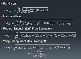
Part of the reason was that the claimed efficiency improvements of the Parkinson, Garman–Klass and other estimators failed to translate into practice when applied to real data. Or, at least, no one could quite be sure whether such estimators really were superior when applied to empirical data since volatility, the second moment of the returns distribution, is inherently unknowable. You can say for sure what the return on a particular stock in a particular month was simply by taking the log of the ratio of the stock price at the month end and beginning. But the same cannot be said of volatility: the standard deviation of daily returns during the month, often naively assumed to represent the asset volatility, is in fact only an estimate of it.
Realized Volatility
All that began to change around 2000 with the advent of high frequency data and the concept of Realized Volatility developed by Andersen and others (see Andersen, T.G., T. Bollerslev, F.X. Diebold and P. Labys (2000), “The Distribution of Exchange Rate Volatility,” Revised version of NBER Working Paper No. 6961). The researchers showed that, in principle, one could arrive at an estimate of volatility arbitrarily close to its true value by summing the squares of asset returns at sufficiently high frequency. From this point onwards, Realized Volatility became the “gold standard” of volatility estimation, leaving other estimators in the dust.
Except that, in practice, there are often reasons why Realized Volatility may not be the way to go: for example, high frequency data may not be available for the series, or only for a portion of it; and bid-ask bounce can have a substantial impact on the robustness of Realized Volatility estimates. So even where high frequency data is available, it may still make sense to compute alternative volatility estimators. Indeed, now that a “gold standard” estimator of true volatility exists, it is possible to get one’s arms around the question of the relative performance of other estimators. That was my intent in my research paper on Estimating Historical Volatility, in which I compare the performance characteristics of the Parkinson, Garman–Klass and other estimators relative to the realized volatility estimator. The comparison was made on a number of synthetic GBM processes in which the simulated series incorporated non-zero drift, jumps, and stochastic volatility. A further evaluation was made using an actual data series, comprising 5 minute returns on the S&P 500 in the period from Jan 1988 to Dec 2003.
The findings were generally supportive of the claimed efficiency improvements for all of the estimators, which were superior to the classical standard deviation of returns on every criterion in almost every case. However, the evident superiority of all of the estimators, including the Realized Volatility estimator, began to decline for processes with non-zero drift, jumps and stochastic volatility. There was even evidence of significant bias in some of the estimates produced for some of the series, notably by the standard deviation of returns estimator.
The Log Volatility Estimator
Finally, analysis of the results from the study of the empirical data series suggested that there were additional effects in the empirical data, not seen in the simulated processes, that caused estimator efficiency to fall well below theoretical levels. One conjecture is that long memory effects, a hallmark of most empirical volatility processes, played a significant role in that finding.
The bottom line is that, overall, the log-range volatility estimator performs robustly and with superior efficiency to the standard deviation of returns estimator, regardless of the precise characteristics of the underlying process.