How to Beat Buy-and-Hold with Less Risk
What is Market Timing? – Common Misconceptions
Market timing has a very bad press and for good reason: the inherent randomness of markets makes reliable forecasting virtually impossible. So why even bother to write about it? The answer is, because market timing has been mischaracterized and misunderstood. It isn’t about forecasting. If fact, with notable exceptions, most of trading isn’t about forecasting. It’s about conditional expectations.
Conditional expectations refer to the expected value of a random variable (such as future stock returns) given certain known information or conditions.
In the context of trading and market timing, it means that rather than attempting to forecast absolute price levels, we base our expectations for future returns on current observable market conditions.
For example, let’s say historical data shows that when the market has declined a certain percentage from its recent highs (condition), forward returns over the next several days tend to be positive on average (expectation). A trading strategy could use this information to buy the dip when that condition is met, not because it is predicting that the market will rally, but because history suggests a favorable risk/reward ratio for that trade under those specific circumstances.
The key insight is that by focusing on conditional expectations, we don’t need to make absolute predictions about where the market is heading. We simply assess whether the present conditions have historically been associated with positive expected returns, and use that probabilistic edge to inform our trading decisions.
This is a more nuanced and realistic approach than binary forecasting, as it acknowledges the inherent uncertainty of markets while still allowing us to make intelligent, data-driven decisions. By aligning our trades with conditional expectations, we can put the odds in our favor without needing a crystal ball.
So, when a market timing algorithm suggests buying the market, it isn’t making a forecast about what the market is going to do next. Rather, what it is saying is, if the market behaves like this then, on past experience, the following trade is likely to be profitable. That is a very different thing from forecasting the market.
A good example of a simple market-timing algorithm is “buying the dips”. It’s so simple that you don’t need a computer algorithm to do it. But a computer algorithm helps by determining what comprises a dip and the level at which profits should be taken.
An Effective Market Timing Strategy
One of my favorites market timing strategies is the following algorithm, which I originally developed to trade the SPY ETF. The equity curve from inception of the ETF in 1993 looks like this:
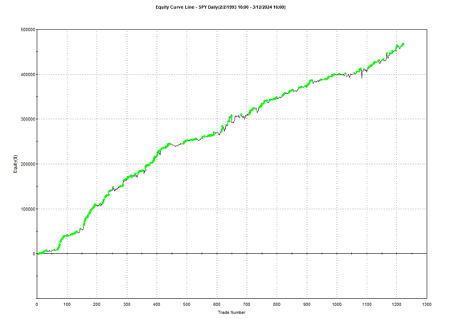
The algorithm combines a few simple technical indicators to determine what constitutes a dip and the level at which profits should be taken. The entry and exit orders are also very straightforward, buying and selling at the market open, which can be achieved by participating in the opening auction. This is very convenient: a signal is generated after the close on day 1 and is then executed as a MOA (market opening auction) order in the opening auction on day 2. The opening auction is by no means the most liquid period of the trading session, but in an ETF like SPY the volumes are such that the market impact is likely to be negligible for the great majority of investors. This is not something you would attempt to do in an illiquid small-cap stock, however, where entries and exits are more reliably handled using a VWAP algorithm; but for any liquid ETF or large-cap stock the opening auction will typically be fine.
Adapting the Strategy to Other Assets and Markets
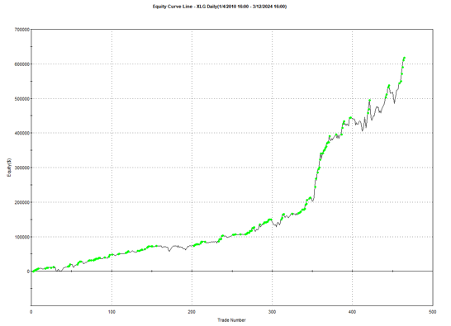
Another aspect that gives me confidence in the algorithm is that it generalizes well to other assets and even other markets. Here, for example, is the equity curve for the exact same algorithm implemented in the XLG ETF in the period from 2010:
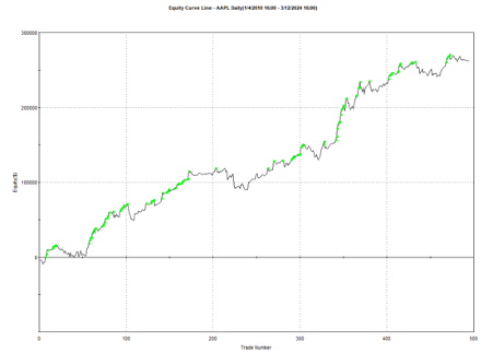
And here is the equity curve for the same strategy (with the same parameters) in AAPL, over the same period:
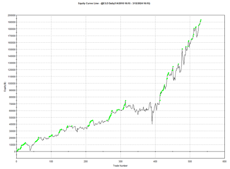
Remarkably, the strategy also works in E-mini futures too, which is highly unusual: typically the market dynamics of the futures market are so different from the spot market that strategies don’t transfer well. But in this case, it simply works:
Understanding Why the Strategy Works
The reason the strategy is effective is due to the upward drift in equities and related derivatives. If you tried to apply a similar strategy to energy or currency markets, it would fail. The strategy’s “secret sauce” is the combination of indicators it uses to determine the short-term low in the ETF that constitutes a good buying opportunity, and then figure out the right level at which to sell.
Does the algorithm always work? If by that you mean “is every trade profitable?” the answer is no. Around 61% of trades are profitable, so there are many instances where trades are closed at a loss. But the net impact of using the market-timing algorithm is very positive, when compared to the buy-and-hold benchmark, as we shall see shortly.
Because the underlying thesis is so simple (i.e. equity markets have positive drift), we can say something about the long-term prospects for the strategy. Equity markets haven’t changed their fundamental tendency to appreciate over the 31-year period from inception of the SPY ETF in 1993, which is why the strategy has performed well throughout that time. Could one envisage market conditions in which the strategy will perform poorly? Yes – any prolonged period of flat to downward trending prices in equities will result in poor performance. But we haven’t seen those conditions since the early 1970’s and, arguably, they are unlikely to return, since the fundamental change brought about by abandonment of the gold standard in 1973.
The abandonment of the gold standard and the subsequent shift to fiat currencies has given central banks, particularly the U.S. Federal Reserve, unprecedented power to expand the money supply and support asset prices during times of crisis. This ‘Fed Put’ has been a major factor underpinning the multi-decade bull market in stocks.
In addition, the increasing dominance of the U.S. as the world’s primary economic and military superpower since the end of the Cold War has made U.S. financial assets a uniquely attractive destination for global capital, creating sustained demand for U.S. equities.
Technological innovation, particularly with respect to the internet and advances in computing, has also unleashed a wave of productivity and wealth creation that has disproportionately benefited the corporate sector and equity holders. This trend shows no signs of abating and may even be accelerating with the advent of artificial intelligence.
While risks certainly remain and occasional cyclical bear markets are inevitable, the combination of accommodative monetary policy, the U.S.’s global hegemony, and technological progress create a powerful set of economic forces that are likely to continue propelling equity prices higher over the long-term, albeit with significant volatility along the way.Strategy Performance in Bear Markets
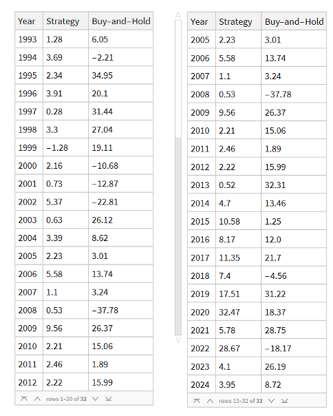
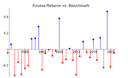
Note that the conditions I am referring to are something unlike anything we have seen in the last 50 years, not just a (serious) market pullback. If we look at the returns in the period from 2000-2002, for example, we see that the strategy held up very well, out-performing the benchmark by 54% over the three-year period of the market crash. Likewise, in 2008 credit crisis, the strategy was able to eke out a small gain, beating the benchmark by over 38%. In fact, the strategy is positive in all but one of the 31 years from inception.
Comparing Performance to Buy-and-Hold
Let’s take a look at the compound returns from the strategy vs. the buy-and-hold benchmark:
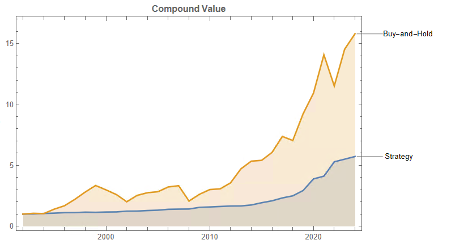
At first sight, it appears that the benchmark significantly out-performs the strategy, albeit suffering from much larger drawdowns. But that doesn’t give an accurate picture of relative performance. To see why, let’s look at the overall performance characteristics:

Now we see that, while the strategy CAGR is 3.50% below the buy-and-hold return, its annual volatility is less than half that of the benchmark, giving the strategy a superior Sharpe Ratio.
Leveraging the Strategy to Enhance Risk-Adjusted Returns
To make a valid comparison between the strategy and its benchmark we therefore need to equalize the annual volatility of both, and we can achieve this by leveraging the strategy by a factor of approximately 2.32. When we do that, we obtain the following results:

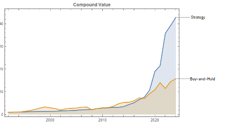
Now that the strategy and benchmark volatilities have been approximately equalized through leverage, we see that the strategy substantially outperforms buy-and-hold by around 355 basis points per year and with far smaller drawdowns.
In general, we see that the strategy outperformed the benchmark in fewer than 50% of annual periods since 1993. However, the size of the outperformance in years when it beat the benchmark was frequently very substantial:
Conclusion
Market timing can work. To understand why, we need to stop thinking in terms of forecasting and think instead about conditional returns. When we do that, we arrive at the insight that market timing works because it relies on the positive drift in equity markets, which has been one of the central features of that market over the last 50 years and is likely to remain so in the foreseeable future. We have confidence in that prediction, because we understand the economic factors that have continued to drive the upward drift in equities over the last half-century.
After that, it is simply a question of the mechanics – how to time the entries and exits. This article describes just one approach amongst a great number of possibilities.
One of the many benefits of market timing is that it has a tendency to side-step the worst market conditions and can produce positive returns even in the most hostile environments: periods such as 2000-2002 and 2008, for example, as we have seen.
Finally, don’t forget that, as we are sitting out of the market approximately 40% of the time our overall risk is much lower – less than half that of the benchmark. So, we can afford to leverage our positions without taking on more overall risk than when we buy and hold. This clearly demonstrates the ability of the strategy to produce higher rates of risk-adjusted return.

