Beta Convexity

What is a Stock Beta?

Around a quarter of a century ago I wrote a paper entitled “Equity Convexity” which – to my disappointment – was rejected as incomprehensible by the finance professor who reviewed it.  But perhaps I should not have expected more: novel theories are rarely well received first time around.  I remain convinced the idea has merit and may perhaps revisit it in these pages at some point in future.  For now, I would like to discuss a related, but simpler concept: beta convexity.  As far as I am aware this, too, is new.  At least, while I find it unlikely that it has not already been considered, I am not aware of any reference to it in the literature.

SSALGOTRADING AD

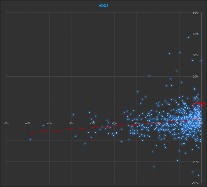
We begin by reviewing the elementary concept of an asset beta, which is the covariance of the return of an asset with the return of the benchmark market index, divided by the variance of the return of the benchmark over a certain period:

Beta formula

Asset betas typically exhibit time dependency and there are numerous methods that can be used to model this feature, including, for instance, the Kalman Filter:


http://jonathankinlay.com/2015/02/statistical-arbitrage-using-kalman-filter/

Beta Convexity

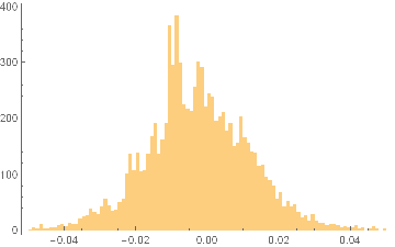
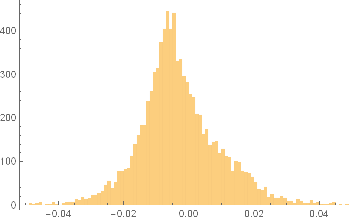
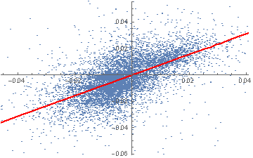
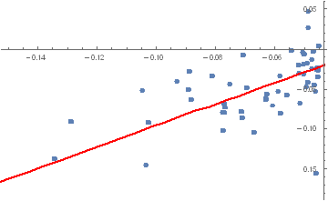
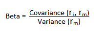
In the context discussed here we set such matters to one side.  Instead of considering how an asset beta may vary over time, we look into how it might change depending on the direction of the benchmark index.  To take an example, let’s consider the stock Advaxis, Inc. (Nasdaq: ADXS).  In the charts below we examine the relationship between the daily stock returns and the returns in the benchmark Russell 3000 Index when the latter are positive and negative.


ADXS - Up Beta ADXS - Down Beta


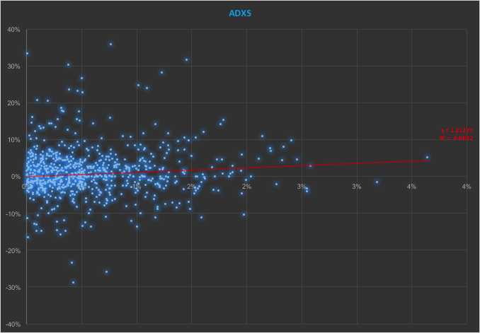
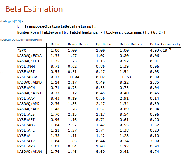
The charts indicate that the stock beta tends to be higher during down periods in the benchmark index than during periods when the benchmark return is positive.  This can happen for two reasons: either the correlation between the asset and the index rises, or the volatility of the asset increases, (or perhaps both) when the overall market declines.  In fact, over the period from Jan 2012 to May 2017, the overall stock beta was 1.31, but the up-beta was only 0.44 while the down-beta was 1.53.  This is quite a marked difference and regardless of whether the change in beta arises from a change in the correlation or in the stock volatility, it could have a significant impact on the optimal weighting for this stock in an equity portfolio.

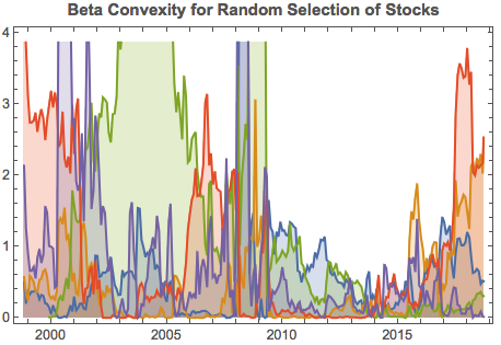
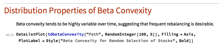
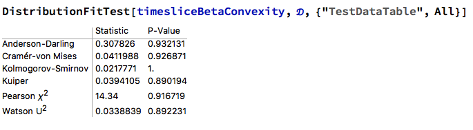
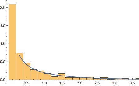
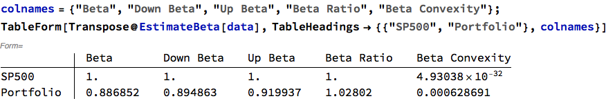
Ideally, what we would prefer to see is very little dependence in the relationship between the asset beta and the sign of the underlying benchmark.  One way to quantify such dependency is with what I have called Beta Convexity:

Beta Convexity = (Up-Beta – Down-Beta) ^2

A stock with a stable beta, i.e. one for which the difference between the up-beta and down-beta is negligibly small, will have a beta-convexity of zero. One the other hand, a stock that shows instability in its beta relationship with the benchmark will tend to have relatively large beta convexity.


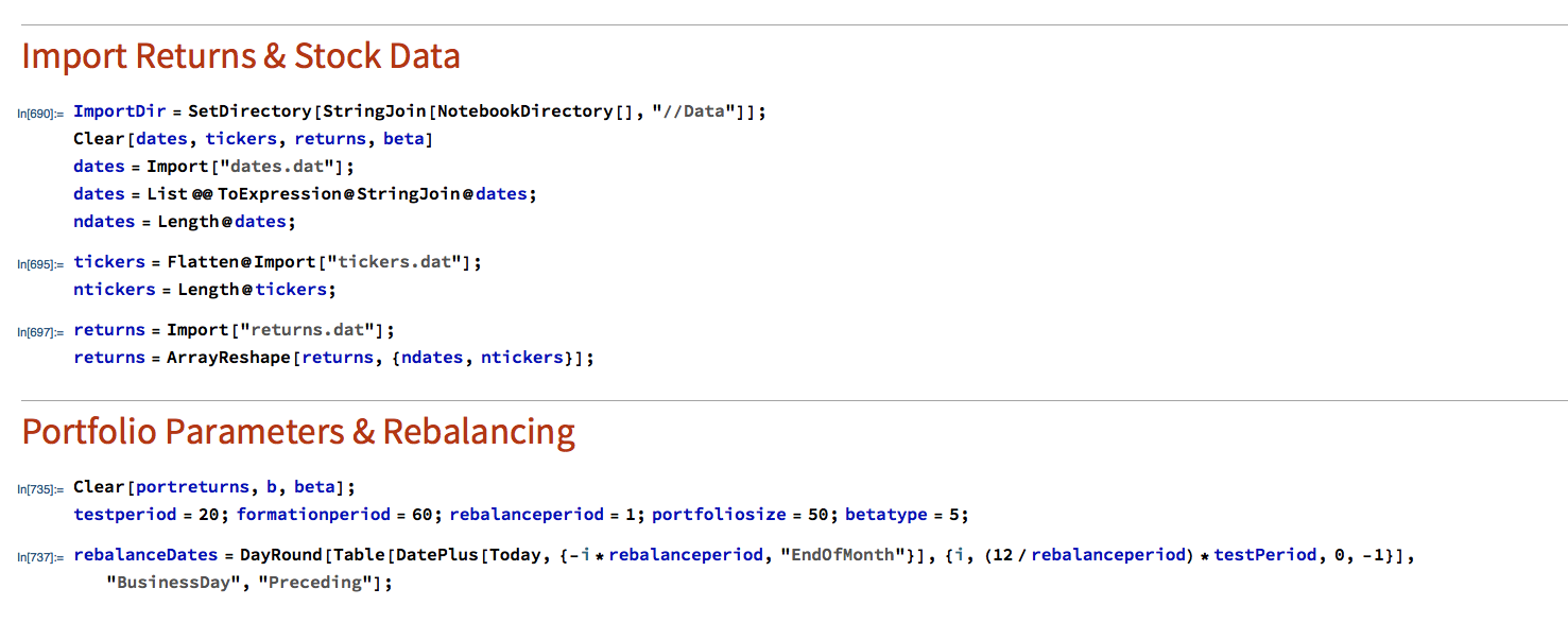
Index Replication using a Minimum Beta-Convexity Portfolio

One way to apply this concept it to use it as a means of stock selection.  Regardless of whether a stock’s overall beta is large or small, ideally we want its dependency to be as close to zero as possible, i.e. with near-zero beta-convexity.  This is likely to produce greater stability in the composition of the optimal portfolio and eliminate unnecessary and undesirable excess volatility in portfolio returns by reducing nonlinearities in the relationship between the portfolio and benchmark returns.

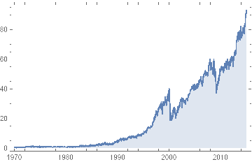
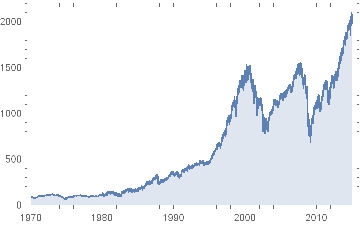
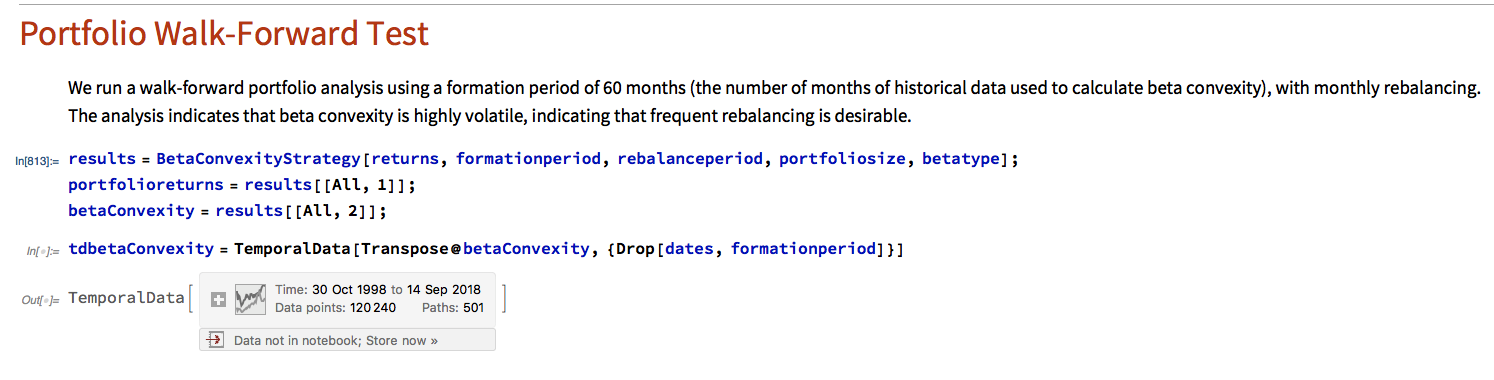
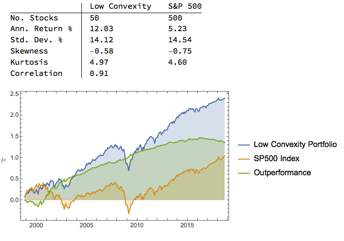
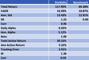
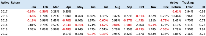
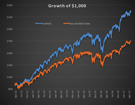
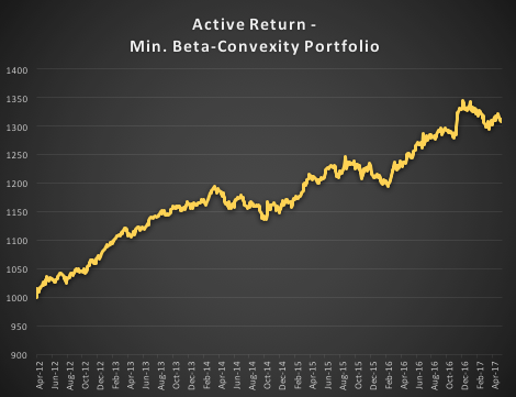
In the following illustration we construct a stock portfolio by choosing the 500 constituents of the benchmark Russell 3000 index that have the lowest beta convexity during the previous 90-day period, rebalancing every quarter (hence all of the results are out-of-sample).  The minimum beta-convexity portfolio outperforms the benchmark by a total of 48.6% over the period from Jan 2012-May 2017, with an annual active return of 5.32% and Information Ratio of 1.36.  The portfolio tracking error is perhaps rather too large at 3.91%, but perhaps can be further reduced with the inclusion of additional stocks.


ResultsTable


Active Monthly


G1000


Active

Conclusion:  Beta Convexity as a New Factor

Beta convexity is a new concept that appears to have a useful role to play in identifying stocks that have stable long term dependency on the benchmark index and constructing index tracking portfolios capable of generating appreciable active returns.

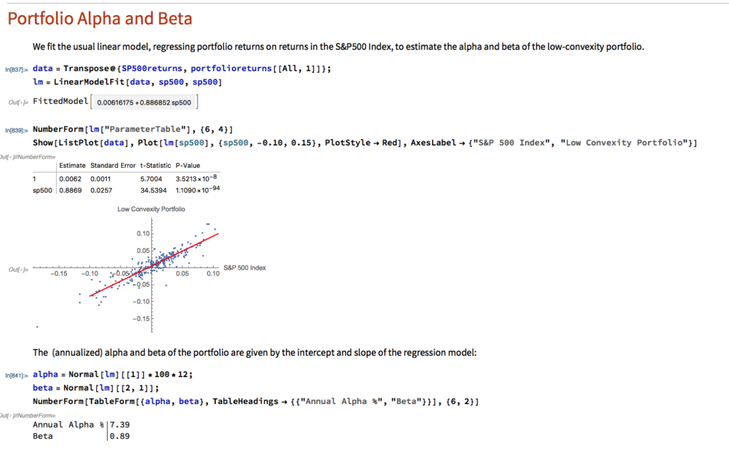
The outperformance of the minimum-convexity portfolio is not the result of a momentum effect, or a systematic bias in the selection of high or low beta stocks.  The selection of the 500 lowest beta-convexity stocks in each period is somewhat arbitrary, but illustrates that the approach can scale to a size sufficient to deploy hundreds of millions of dollars of investment capital, or more.  A more sensible scheme might be, for example, to select a variable number of stocks based on a predefined tolerance limit on beta-convexity.

Obvious steps from here include experimenting with alternative weighting schemes such as value or beta convexity weighting and further refining the stock selection procedure to reduce the portfolio tracking error.

Further useful applications of the concept are likely to be found in the design of equity long/short and  market neural strategies. These I shall leave the reader to explore for now, but I will perhaps return to the topic in a future post.

Crash-Protecting Your Portfolio With CrashMetrics

In a post on LinkedIn I referred to the concept of CrashMetrics and how it can be used for portfolio protection.  It’s a simple approach to the management of extreme risk that works rather well.  It can be summarized as “CAPM for crashes”.  Here’s how it works.

Let’s take Proctor and Gamble as our example stock.  We’ll use daily data from 1970-2014 for the stock and for the S&P 500 Index, as follows:

DateListPlot[PG=TimeSeries[FinancialData[“PG”,{{1970,1,2},{2014,12,31}}]],Filling->Axis]

PG 1970-2014


DateListPlot[SP500=TimeSeries[FinancialData[“^GSPC”,{{1970,1,2},{2014,12,31}}]],Filling->Axis]

SP500 Index 1970-2014


We are also going to need an estimate of the risk free rate of return.  We’ll use a 30-day T-Bill rate:

DateListPlot[TBill=TimeSeries[FinancialData[“^IRX”,{{1970,1,2},{2014,12,31}}]],Filling->Axis]

TBill 1970-2014

CAPM Beta Estimation

Next we convert the annual Bill yields into estimates of the continuously compounded daily return and subtract these from the gross returns for PG and the S&P 500 Index, to create series of excess returns for the stock and the index.

 SP500Dates=SP500[“Times”]
PGReturns=Log[PG[Drop[SP500Dates,1]]]-Log[PG[Drop[SP500Dates,-1]]];
SP500Returns=Log[Drop[SP500[“Values”],1]]-Log[Drop[SP500[“Values”],-1]];
TBillDailyRate=Log[TBill[Drop[SP500Dates,1]]]/250 /. Indeterminate->0;
Histogram[PGXReturns=PGReturns-TBillDailyRate,{-0.05,0.05,0.001}]

PG Excess Returns Hist

Excess Returns PG 1970-2014

SP500 Index Excess Returns Hist

Excess Returns S&P 500 Index 1970-2014

We are now ready to estimate the stock beta for PG, using a simple linear regression model of the excess returns in the stock vs. the excess returns in the S&P 500 Index:

 dataset=Partition[Riffle[SP500XReturns,PGXReturns],2
CAPM = LinearModelFit[dataset,x,x]

CAPM Model

From which we estimate the  beta for PG to be around 0.78 (the slope of the regression line in the scatterplot below).  That seems plausible for a large, diversified consumer goods manufacturer, which is likely to be less volatile than the broad index during normal market conditions.

 Show[ListPlot[dataset],Plot[CAPM[x],{x,-0.05,0.05},PlotStyle->Red]]

CAPM Scatterplot

The CAPM regression shows that around 40% of the variation in excess returns in PG is explained by movements in the broad market (the remainder is due to stock-specific risk factors):

 CAPM[“AdjustedRSquared”] = 0.40

That’s a typically scenario with the CAPM model, which is based on some fairly simple, but rather heroic assumptions that we need not delve too deeply into here.

CrashMetrics Approach

In CrashMetrics we focus exclusively in the left tail of the distribution.  For the S&P 500 index the average excess return is very close to zero, while the daily standard deviation of returns is just over 1.5%.  So let’s focus on down-moves that are, say, at least 3xSD, or larger.  We create a reduced data set comprising days on which the index declined by at least 4.5%, and repeat the regression procedure using just those 54 days:

 Dimensions[reducedDataset=Select[dataset,#[[1]] < -0.045&]{54,2}

 CrashM = LinearModelFit[reducedDataset,x,x]

CrashM Model

 Show[ListPlot[reducedDataset],Plot[CrashM[x],{x,0, -0.25},PlotStyle->Red]]

CrashM Scatterplot

Two points are especially noteworthy.

The first is that the beta for PG during major market down-moves is a lot higher than during normal markets (around 1.34 vs 0.78) and being greater than 1, indicates that during adverse conditions PG tends to exacerbate the down-turn in the broad market.

The second is that the regression R-squared is much higher (0.68) for the CrashMetrics regression model, reflecting the tendency of stocks to correlate more closely with the market index during major sell-offs. In that sense, the “crash-beta” estimate is a more reliable estimate than the regular CAPM beta.

How to Use CrashMetrics

How is this technique helpful to the portfolio manager?

To begin, you might want to estimate crash-betas for all of the stocks in your portfolio and for the portfolio as a whole, to give you a handle on how the portfolio is likely to behave under extreme stress.

You could then choose to make adjustments to the portfolio composition to reduce its crash exposure.  This can be done by reducing the allocations to high crash-beta stocks in favor of low crash-beta stocks.  Alternatively, you can buy tail protection using out-of-the-money put options in high-crash beta stocks.  What’s interesting about this technique is that you might end up paying less for crash-protection than you might think.

Taking our PG test case as an example, this is typically seen as a less risky stock and its options are priced accordingly.  Consequently, the Gamma in the options looks cheap when considering how the stock behaves during market crashes.  Conversely, options in very volatile stocks (AAPL springs  to mind, for example), are likely to be relatively highly priced, but may offer less protection during a crash scenario, depending on the behavior of the stock during major market declines.


Beating the S&P500 Index with a Low Convexity Portfolio

What is Beta Convexity?

Beta convexity is a measure of how stable a stock beta is across market regimes.  The essential idea is to evaluate the beta of a stock during down-markets, separately from periods when the market is performing well.  By choosing a portfolio of stocks with low beta-convexity we seek to stabilize the overall risk characteristics of our investment portfolio.

A primer on beta convexity and its applications is given in the following post:


In this post I am going to use the beta-convexity concept to construct a long-only equity portfolio capable of out-performing the benchmark S&P 500 index.

The post is in two parts.  In the first section I outline the procedure in Mathematica for downloading data and creating a matrix of stock returns for the S&P 500 membership.  This is purely about the mechanics, likely to be of interest chiefly to Mathematica users. The code deals with the issues of how to handle stocks with multiple different start dates and missing data, a problem that the analyst is faced with on a regular basis.  Details are given in the pdf below. Let’s skip forward to the analysis.

Portfolio Formation & Rebalancing

We begin by importing the data saved using the data retrieval program, which comprises a matrix of (continuously compounded) monthly returns for the S&P500 Index and its constituent stocks.  We select a portfolio size of 50 stocks, a test period of 20 years, with a formation period of 60 months and monthly rebalancing.

In the processing stage, for each month in our 20-year test period we  calculate the beta convexity for each index constituent stock and select the 50 stocks that have the lowest beta-convexity during the prior 5-year formation period.  We then compute the returns for an equally weighted basket of the chosen stocks over the following month.  After that, we roll forward one month and repeat the exercise.

It turns out that beta-convexity tends to be quite unstable, as illustrated for a small sample of component stocks in the chart below:

A snapshot of estimated convexity factors is shown in the following table.  As you can see, there is considerable cross-sectional dispersion in convexity, in addition to time-series dependency.

At any point in time the cross-sectional dispersion is well described by a Weibull distribution, which passes all of the usual goodness-of-fit tests.

Performance Results

We compare the annual returns and standard deviation of the low convexity portfolio with the S&P500 benchmark in the table below. The results indicate that the average gross annual return of a low-convexity portfolio of 50 stocks is more than double that of the benchmark, with a comparable level of volatility. The portfolio also has slightly higher skewness and kurtosis than the benchmark, both desirable characteristics.


Portfolio Alpha & Beta Estimation

Using the standard linear CAPM model we estimate the annual alpha of the low-convexity portfolio to be around 7.39%, with a beta of 0.89.

Beta Convexity of the Low Convexity Portfolio

As we might anticipate, the beta convexity of the portfolio is very low since it comprises stocks with the lowest beta-convexity:

Conclusion: Beating the Benchmark S&P500 Index

Using a beta-convexity factor model, we are able to construct a small portfolio that matches the benchmark index in terms of volatility, but with markedly superior annual returns.  Larger portfolios offering greater liquidity produce slightly lower alpha, but a 100-200 stock portfolio typically produce at least double the annual rate of return of the benchmark over the 20-year test period.

For those interested, we shall shortly be offering a low-convexity strategy on our Systematic Algotrading platform – see details below:

Section on Data Retrieval and Processing

Data Retrieval