Continuing a previous post, in which we modeled the relationship in the levels of the VIX Index and the Year 1 and Year 2 CBOE Correlation Indices, we next turn our attention to modeling changes in the VIX index.
In case you missed it, the post can be found here:
http://jonathankinlay.com/2017/08/correlation-cointegration/
We saw previously that the levels of the three indices are all highly correlated, and we were able to successfully account for approximately half the variation in the VIX index using either linear regression models or non-linear machine-learning models that incorporated the two correlation indices. It turns out that the log-returns processes are also highly correlated:

A Linear Model of VIX Returns
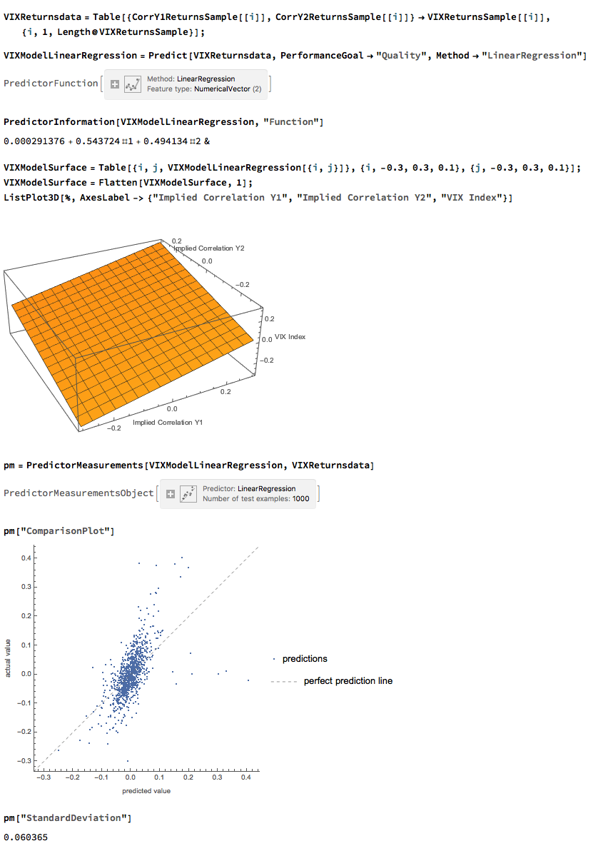
We can create a simple linear regression model that relates log-returns in the VIX index to contemporaneous log-returns in the two correlation indices, as follows. The derived model accounts for just under 40% of the variation in VIX index returns, with each correlation index contributing approximately one half of the total VIX return.

Non-Linear Model of VIX Returns
Although the linear model is highly statistically significant, we see clear evidence of lack of fit in the model residuals, which indicates non-linearities present in the relationship. So, ext we use a nearest-neighbor algorithm, a machine learning technique that allows us to model non-linear components of the relationship. The residual plot from the nearest neighbor model clearly shows that it does a better job of capturing these nonlinearities, with lower standard in the model residuals, compared to the linear regression model:

Correlation Copulas
Another approach entails the use of copulas to model the inter-dependency between the volatility and correlation indices. For a fairly detailed exposition on copulas, see the following blog posts:
http://jonathankinlay.com/2017/01/copulas-risk-management/
http://jonathankinlay.com/2017/03/pairs-trading-copulas/
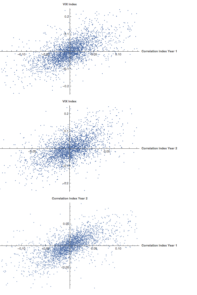
We begin by taking a smaller sample comprising around three years of daily returns in the indices. This minimizes the impact of any long-term nonstationarity in the processes and enables us to fit marginal distributions relatively easily. First, let’s look at the correlations in our sample data:
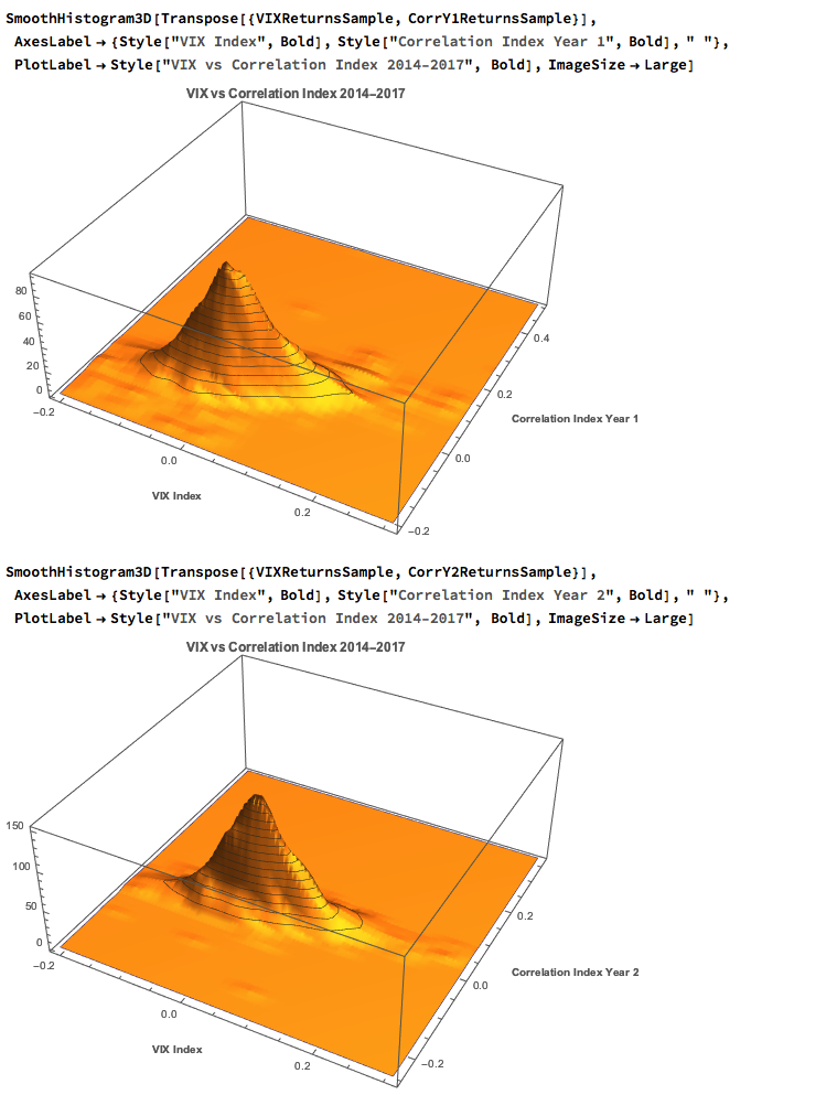
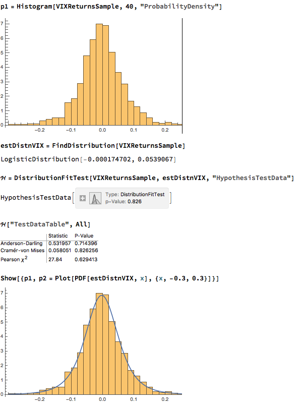
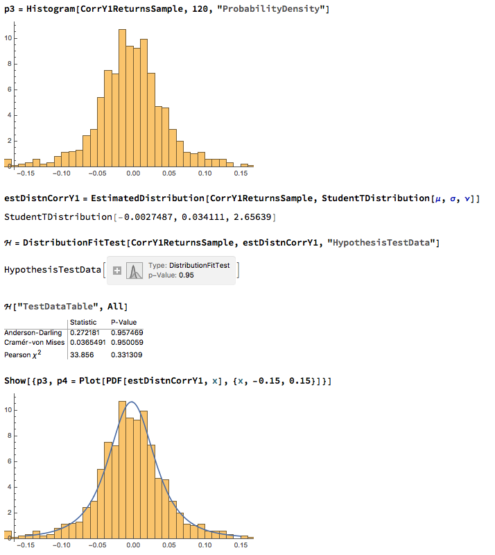
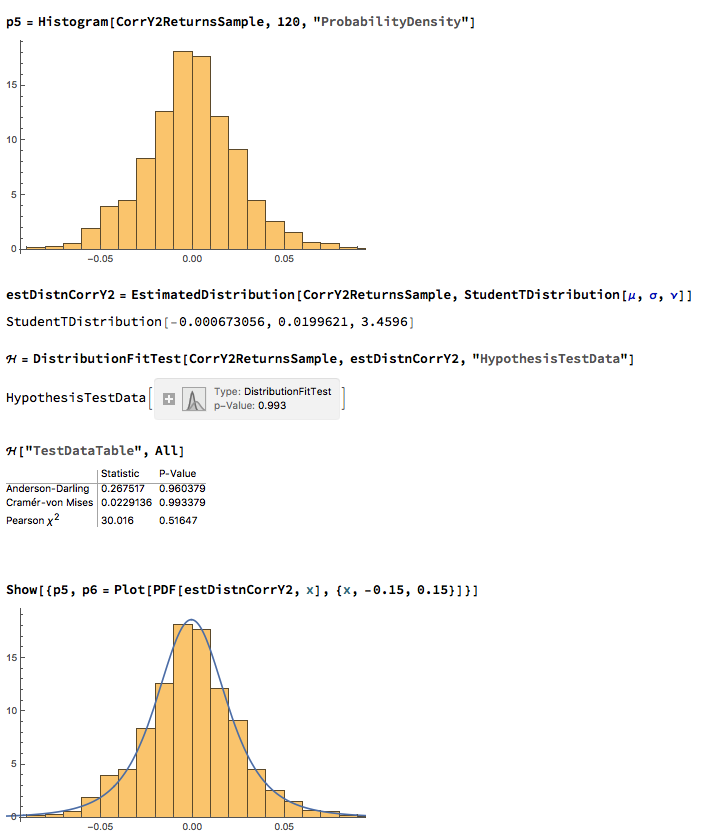
We next proceed to fit margin distributions to the VIX and Correlation Index processes. It turns out that the VIX process is well represented by a Logistic distribution, while the two Correlation Index returns processes are better represented by a Student-T density. In all three cases there is little evidence of lack of fit, wither in the body or tails of the estimated probability density functions:
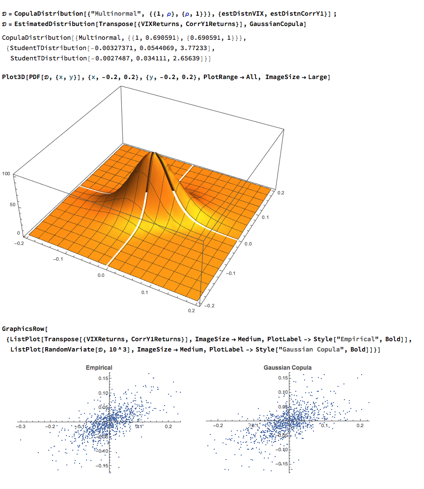
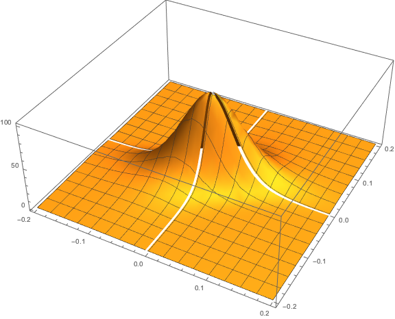
The final step is to fit a copula to model the joint density between the indices. To keep it simple I have chosen to carry out the analysis for the combination of the VIX index with only the first of the correlation indices, although in principle there no reason why a copula could not be estimated for all three indices. The fitted model is a multinormal Gaussian copula with correlation coefficient of 0.69. of course, other copulas are feasible (Clayton, Gumbel, etc), but Gaussian model appears to provide an adequate fit to the empirical copula, with approximate symmetry in the left and right tails.