Emini futures Archives - QUANTITATIVE RESEARCH AND TRADING

January 15, 2019

Signal Processing and Sample Frequency

The Importance of Sample Frequency

Too often we apply a default time horizon for our trading, whether it below (daily, weekly) or higher (hourly, 5 minute) frequency. Sometimes the choice is dictated by practical considerations, such as a desire to avoid overnight risk, or the (lack of0 availability of low-latency execution platform.

But there is an alternative approach to the trade frequency decision that often yields superior results in terms of trading performance. The methodology derives from signal processing and the idea essentially is to use Fourier transforms to help identify the cyclical behavior of the strategy alpha and hence determine the best time-frames for sampling and trading. I wrote about this is a previous blog post, in which I described how to use principal components analysis to investigate the factors driving the returns in various pairs trading strategies. Here I want to take a simpler approach, in which we use Fourier analysis to select suitable sample frequencies. The idea is simply to select sample frequencies where the signal strength appears strongest, in the hope that it will lead to superior performance characteristics in what strategy we are trying to develop.

Signal Decomposition for S&P500 eMini Futures

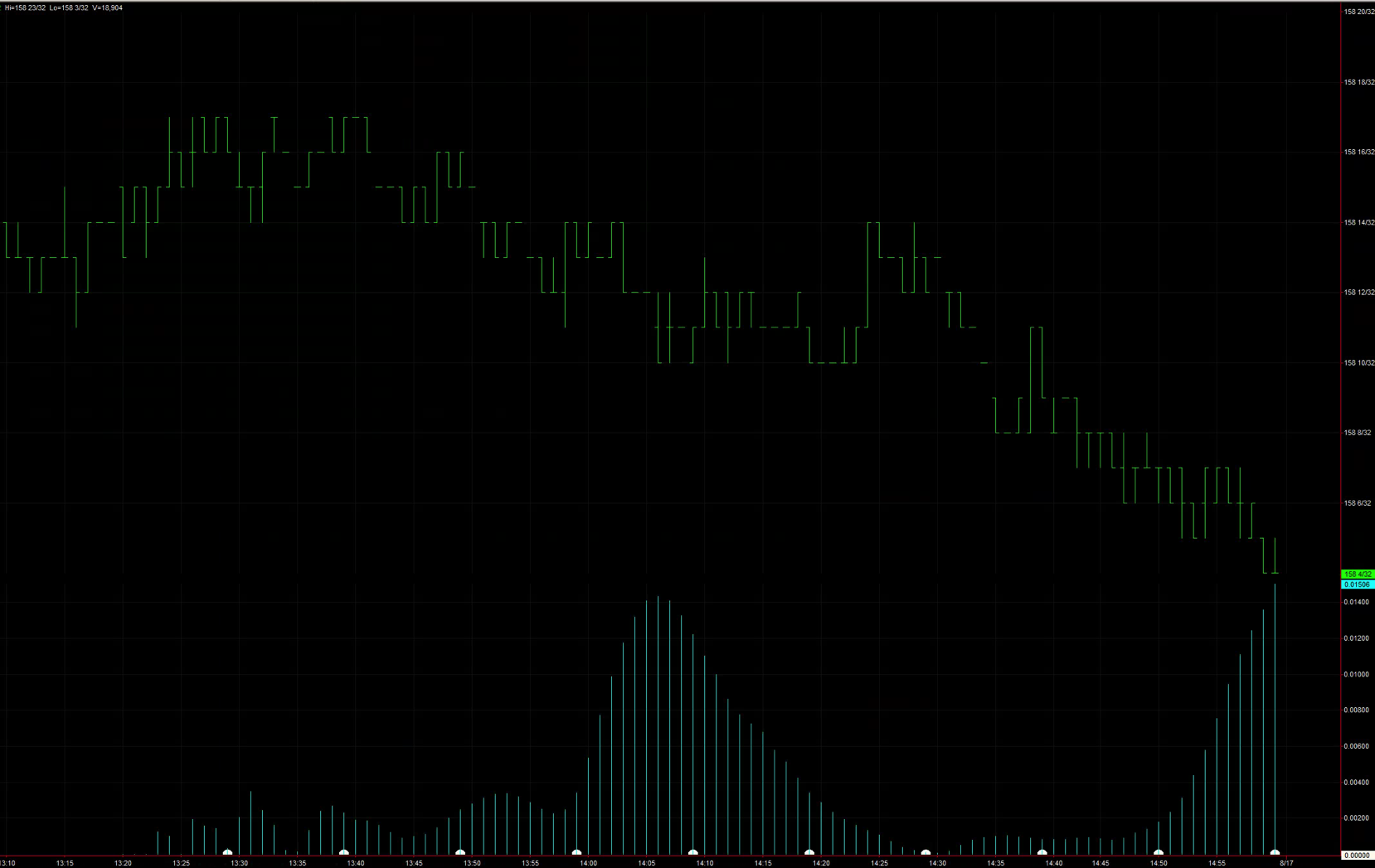
Let’s take as an example the S&P 500 emini futures contract. The chart below shows the continuous ES futures contract plotted at 1-minute intervals from 1998. At the bottom of the chart I have represented the signal analysis as a bar chart (in blue), with each bar representing the amplitude at each frequency. The white dots on the chart identify frequencies that are spaced 10 minutes apart. It is immediately evident that local maxima in the spectrum occur around 40 mins, 60 mins and 120 mins. So a starting point for our strategy research might be to look at emini data sampled at these frequencies. Incidentally, it is worth pointing out that I have restricted the session times to 7AM – 4PM EST, which is where the bulk of the daily volume and liquidity tend to occur. You may get different results if you include data from the Globex session.

This is all very intuitive and unsurprising: the clearest signals occur at frequencies that most traders typically tend to trade, using hourly data, for example. Any strategy developer is already quite likely to consider these and other common frequencies as part of their regular research process. There are many instances of successful trading strategies built on emini data sampled at 60 minute intervals.

Signal Decomposition for US Bond Futures

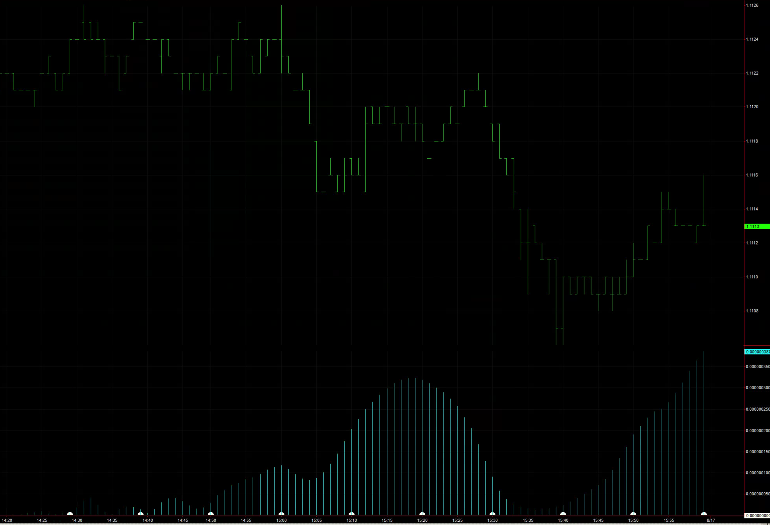
Let’s look at a rather more interesting example: US (30 year) Bond futures. Unlike the emini contract, the spectral analysis of the US futures contract indicates that the strongest signal by far occurs at a frequency of around 47 minutes. This is decidedly an unintuitive outcome – I can’t think of any reason why such a strong signal should appear at this cycle length, but, statistically it does.

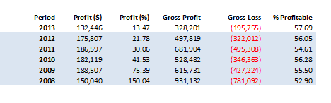
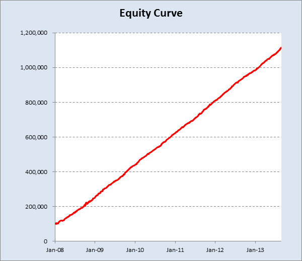
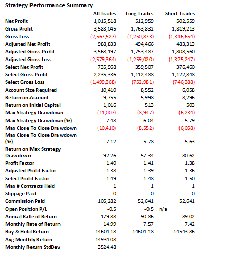
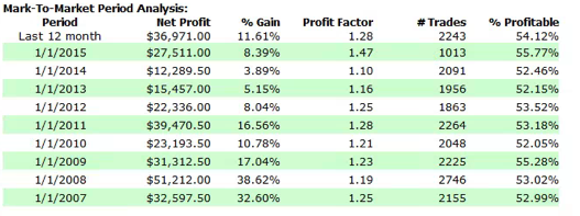
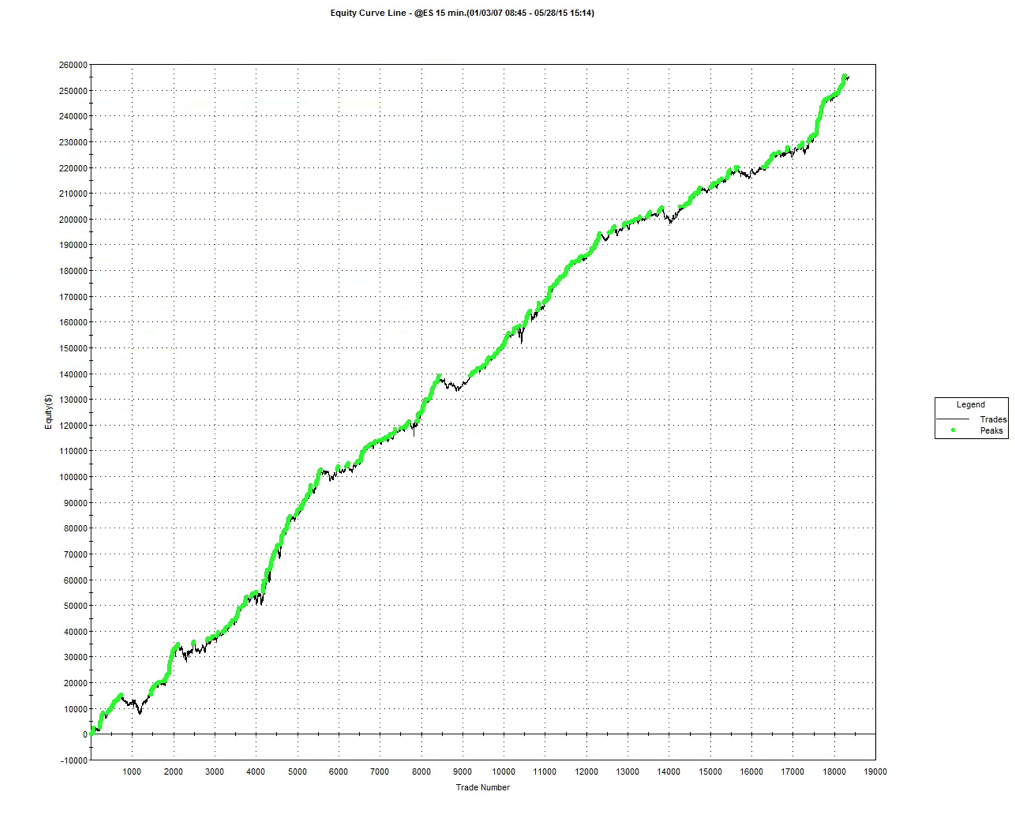
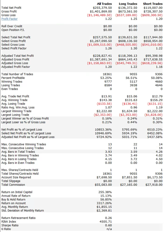
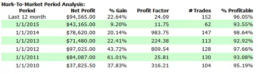
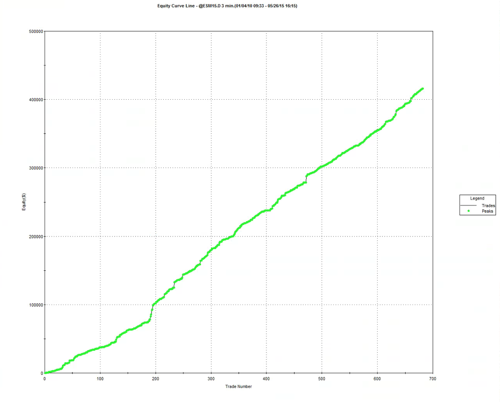
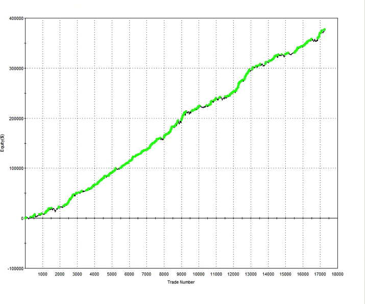
Does it work? Readers can judge for themselves: below is an example of an equity curve for a strategy on US futures sampled at 47 minute frequency over the period from 2002. The strategy has performed very consistently, producing around $25,000 per contract per year, after commissions and slippage.

Conclusion

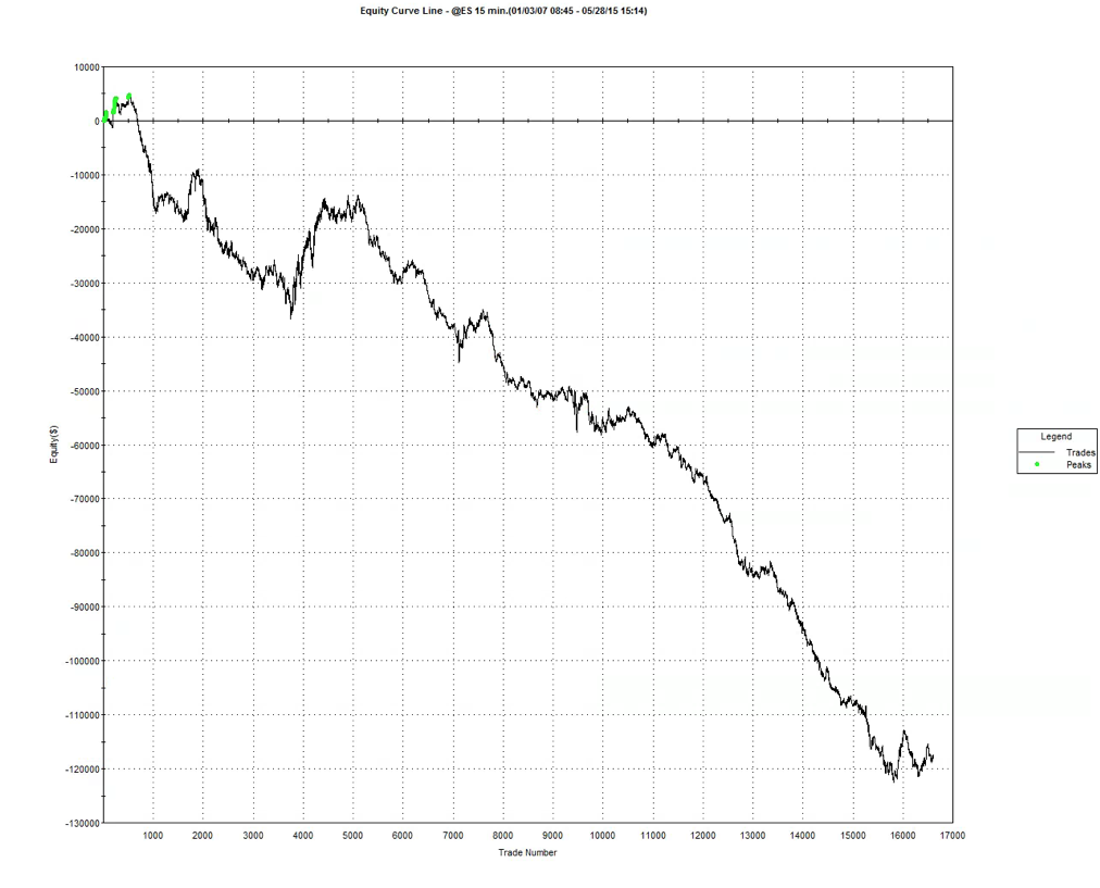
While I have had similar success with products as diverse as Corn and VIX futures, the frequency domain approach is by no means a panacea: there are plenty of examples where I have been unable to construct profitable strategies for data sampled at the frequencies with very strong signals. Conversely, I have developed successful strategies using data at frequencies that hardly registered at all on the spectrum, but which I selected for other reasons. Nonetheless, spectral analysis (and signal processing in general) can be recommended as a useful tool in the arsenal of any quantitative analyst.

December 4, 2018

High Frequency Trading Strategies

Most investors have probably never seen the P&L of a high frequency trading strategy. There is a reason for that, of course: given the typical performance characteristics of a HFT strategy, a trading firm has little need for outside capital. Besides, HFT strategies can be capacity constrained, a major consideration for institutional investors. So it is amusing to see the reaction of an investor on encountering the track record of a HFT strategy for the first time. Accustomed as they are to seeing Sharpe ratios in the range of 0.5-1.5, or perhaps as high as 1.8, if they are lucky, the staggering risk-adjusted returns of a HFT strategy, which often have double-digit Sharpe ratios, are truly mind-boggling.

By way of illustration I have attached below the performance record of one such HFT strategy, which trades around 100 times a day in the eMini S&P 500 contract (including the overnight session). Note that the edge is not that great – averaging 55% profitable trades and profit per contract of around half a tick – these are some of the defining characteristics of HFT trading strategies. But due to the large number of trades it results in very substantial profits. At this frequency, trading commissions are very low, typically under $0.1 per contract, compared to $1 – $2 per contract for a retail trader (in fact an HFT firm would typically own or lease exchange seats to minimize such costs).

Hidden from view in the above analysis are the overhead costs associated with implementing such a strategy: the market data feed, execution platform and connectivity capable of handling huge volumes of messages, as well as algo logic to monitor microstructure signals and manage order-book priority. Without these, the strategy would be impossible to implement profitably.

Scaling things back a little, lets take a look at a day-trading strategy that trades only around 10 times a day, on 15-minute bars. Although not ultra-high frequency, the strategy nonetheless is sufficiently high frequency to be very latency sensitive. In other words, you would not want to try to implement such a strategy without a high quality market data feed and low-latency trading platform capable of executing at the 1-millisecond level. It might just be possible to implement a strategy of this kind using TT’s ADL platform, for example.

While the win rate and profit factor are similar to the first strategy, the lower trade frequency allows for a higher trade PL of just over 1 tick, while the equity curve is a lot less smooth reflecting a Sharpe ratio that is “only” around 2.7.

The critical assumption in any HFT strategy is the fill rate. HFT strategies execute using limit or IOC orders and only a certain percentage of these will ever be filled. Assuming there is alpha in the signal, the P&L grows in direct proportion to the number of trades, which in turn depends on the fill rate. A fill rate of 10% to 20% is usually enough to guarantee profitability (depending on the quality of the signal). A low fill rate, such as would typically be seen if one attempted to trade on a retail trading platform, would destroy the profitability of any HFT strategy.

To illustrate this point, we can take a look at the outcome if the above strategy was implemented on a trading platform which resulted in orders being filled only when the market trades through the limit price. It isn’t a pretty sight.

The moral of the story is: developing a HFT trading algorithm that contains a viable alpha signal is only half the picture. The trading infrastructure used to implement such a strategy is no less critical. Which is why HFT firms spend tens, or hundreds of millions of dollars developing the best infrastructure they can afford.

November 27, 2018

Designing a Scalable Futures Strategy

I have been working on a higher frequency version of the eMini S&P 500 futures strategy, based on 3-minute bar intervals, which is designed to trade a couple of times a week, with hold periods of 2-3 days. Even higher frequency strategies are possible, of course, but my estimation is that a hold period of under a week provides the best combination of liquidity and capacity. Furthermore, the strategy is of low enough frequency that it is not at all latency sensitive – indeed, in the performance analysis below I have assumed that the market must trade through the limit price before the system enters a trade (relaxing the assumption and allowing the system to trade when the market touches the limit price improves the performance).

The other important design criteria are the high % of profitable trades and Kelly f (both over 95%). This enables the investor to employ money management techniques, such a fixed-fractional allocation for example, in order to scale the trade size up from 1 to 10 contracts, without too great a risk of a major drawdown in realized P&L.

The end result is a strategy that produces profits of $80,000 to $100,000 a year on a 10 contract position, with an annual rate of return of 30% and a Sharpe ratio in excess of 2.0.

Furthermore, of the 682 trades since Jan 2010, only 29 have been losers.

Annual P&L (out of sample)

Equity Curve

Strategy Performance

What’s the Downside?

Everything comes at a price, of course. Firstly, the strategy is long-only and, by definition, will perform poorly in falling markets, such as we saw in 2008. That’s a defensible investment thesis, of course – how many $billions are invested in buy and hold strategies? – and, besides, as one commentator remarked, the trick is to develop multiple strategies for different market regimes (although, sensible as that sounds, one is left with the difficulty of correctly identifying the market regime).

The second drawback is revealed by the trade chart below, which plots the drawdown experienced during each trade. The great majority of these drawdowns are unrealized, and in most cases the trade recovers to make a profit. However, there are some very severe cases, such as Sept 2014, when the strategy experienced a drawdown of $85,000 before recovering to make a profit on the trade. For most investors, the agony of risking an entire year’s P&L just to make a few hundred dollars would be too great.

It should be pointed out that the by the time the drawdown event took place the strategy had already produced many hundreds of thousands of dollars of profit. So, one could take the view that by that stage the strategy was playing with “house money” and could well afford to take such a risk.

One obvious “solution” to the drawdown problem is to use some kind of stop loss. Unfortunately, the effect is simply to convert an unrealized drawdown into a realized loss. For some, however, it might be preferable to take a hit of $40,000 or $50,000 once every few years, rather than suffer the uncertainty of an even larger potential loss. Either way, despite its many pleasant characteristics, this is not a strategy for investors with weak stomachs!