High Frequency Trading: Equities vs. Futures

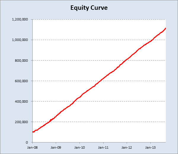
A talented young system developer I know recently reached out to me with an interesting-looking equity curve for a high frequency strategy he had designed in E-mini futures:

Fig1

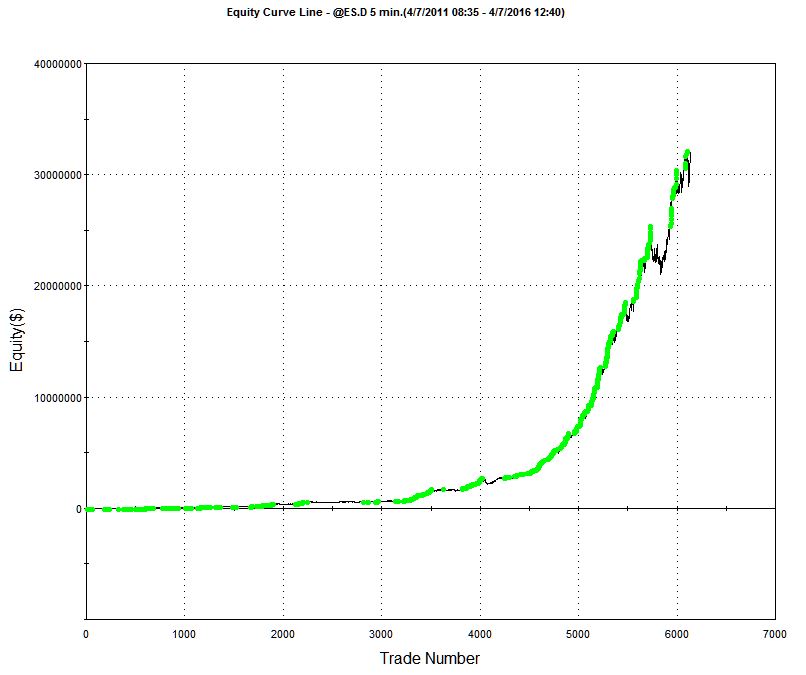
Pretty obviously, he had been making creative use of the “money management” techniques so beloved by futures systems designers.  I invited him to consider how it would feel to be trading a 1,000-lot E-mini position when the market took a 20 point dive.  A $100,000 intra-day drawdown might make the strategy look a little less appealing.  On the other hand, if you had already made millions of dollars in the strategy, you might no longer care so much.

SSALGOTRADING AD

A more important criticism of money management techniques is that they are typically highly path-dependent:  if you had started your strategy slightly closer to one of the drawdown periods that are almost unnoticeable on the chart, it could have catastrophic consequences for your trading account.  The only way to properly evaluate this, I advised, was to backtest the strategy over many hundreds of thousands of test-runs using Monte Carlo simulation.  That would reveal all too clearly that the risk of ruin was far larger than might appear from a single backtest.

Next, I asked him whether the strategy was entering and exiting passively, by posting bids and offers, or aggressively, by crossing the spread to sell at the bid and buy at the offer.  I had a pretty good idea what his answer would be, given the volume of trades in the strategy and, sure enough he confirmed the strategy was using passive entries and exits.  Leaving to one side the challenge of executing a trade for 1,000 contracts in this way, I instead ask him to show me the equity curve for a single contract in the underlying strategy, without the money-management enhancement. It was still very impressive.

Fig2


The Critical Fill Assumptions For Passive Strategies

But there is an underlying assumption built into these results, one that I have written about in previous posts: the fill rate.  Typically in a retail trading platform like Tradestation the assumption is made that your orders will be filled if a trade occurs at the limit price at which the system is attempting to execute.  This default assumption of a 100% fill rate is highly unrealistic.  The system’s orders have to compete for priority in the limit order book with the orders of many thousands of other traders, including HFT firms who are likely to beat you to the punch every time.  As a consequence, the actual fill rate is likely to be much lower: 10% to 20%, if you are lucky.  And many of those fills will be “toxic”:  buy orders will be the last to be filled just before the market  moves lower and sell orders will be the last to get filled just as the market moves higher. As a result, the actual performance of the strategy will be a very long way from the pretty picture shown in the chart of the hypothetical equity curve.

One way to get a handle on the problem is to make a much more conservative assumption, that your limit orders will only get filled when the market moves through them.  This can easily be achieved in a product like Tradestation by selecting the appropriate backtest option:

fig3


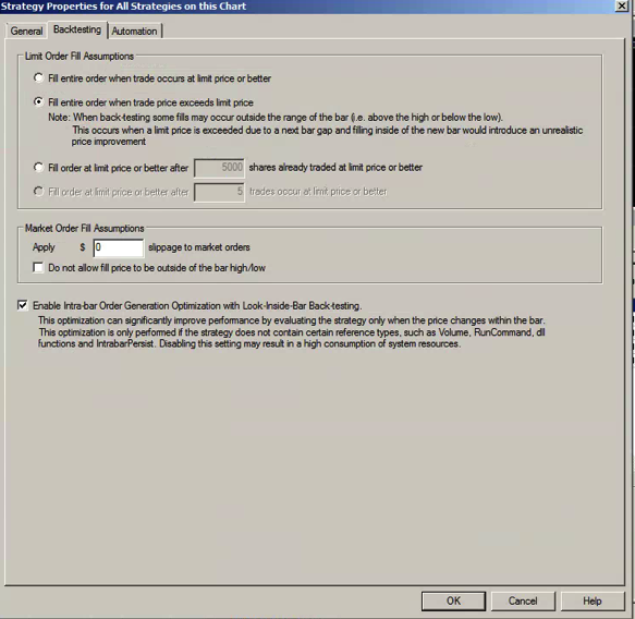
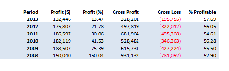
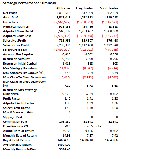
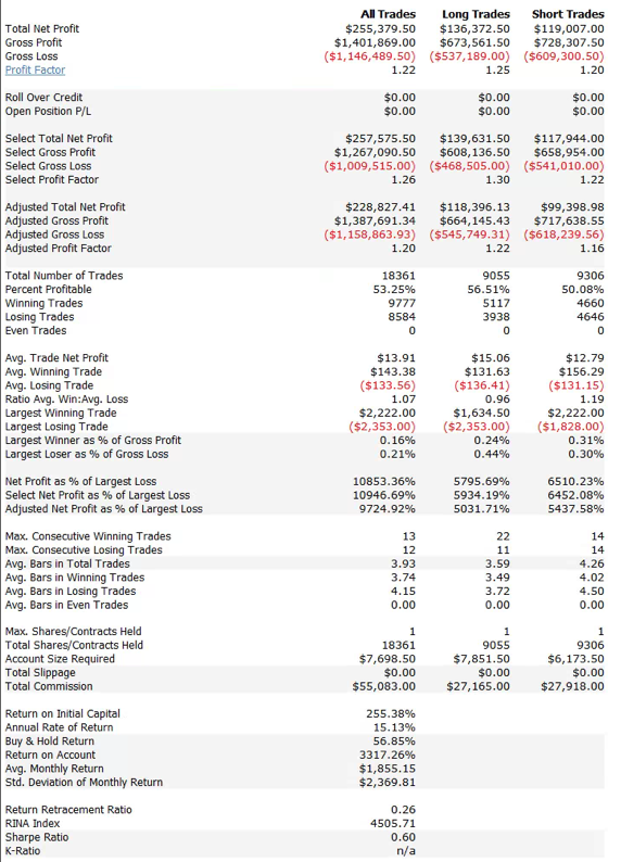
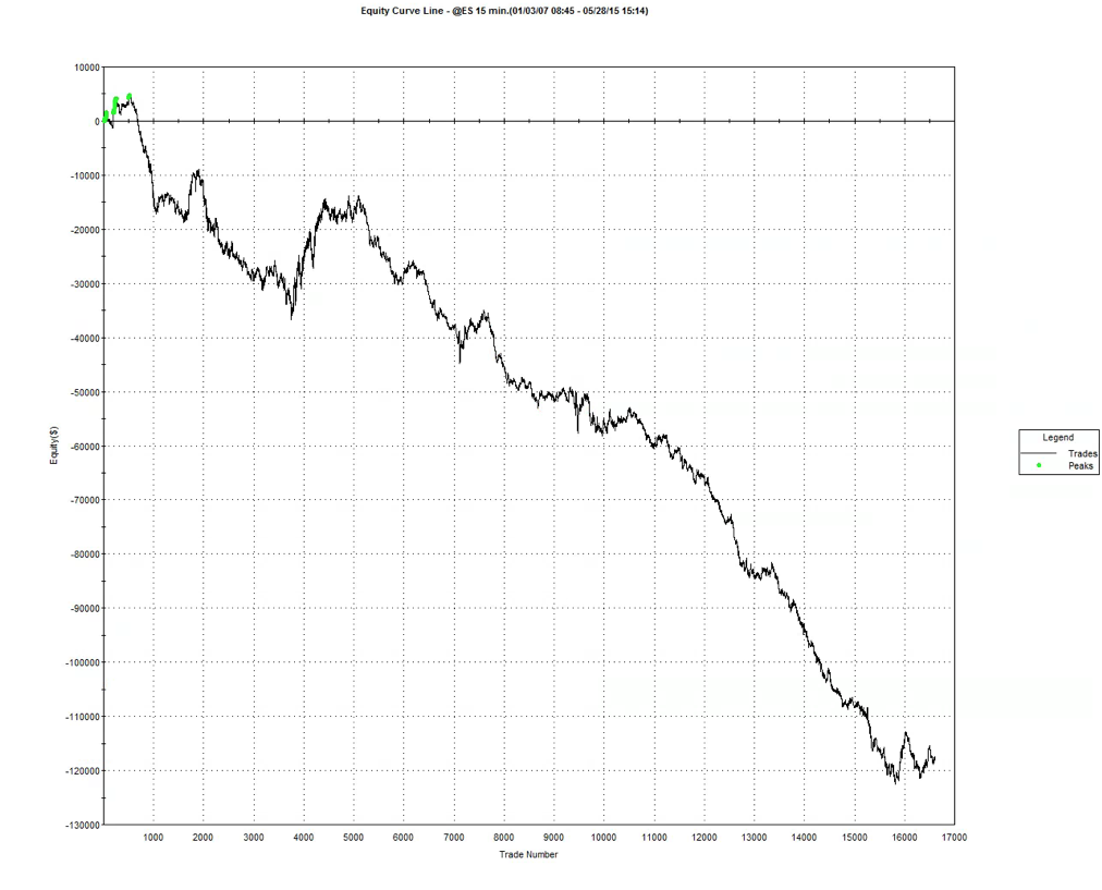
The strategy performance results often look very different when this much more conservative fill assumption is applied.  The outcome for this system was not at all unusual:

Fig4


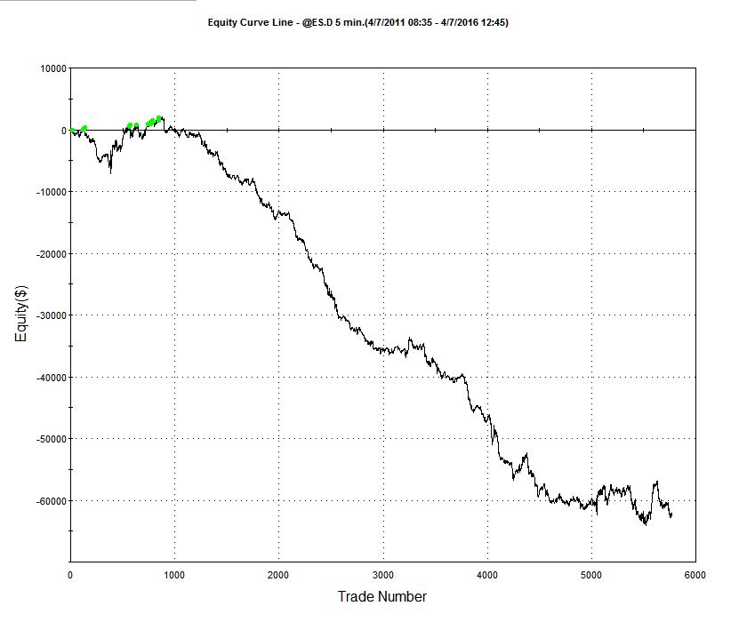
Of course, the more conservative assumption applied here is also unrealistic:  many of the trading system’s sell orders would be filled at the limit price, even if the market failed to move higher (or lower in the case of a buy order).  Furthermore, even if they were not filled during the bar-interval in which they were issued, many limit orders posted by the system would be filled in subsequent bars.  But the reality is likely to be much closer to the outcome assuming a conservative fill-assumption than an optimistic one.    Put another way:  if the strategy demonstrates good performance under both pessimistic and optimistic fill assumptions there is a reasonable chance that it will perform well in practice, other considerations aside.

An Example of a HFT Equity Strategy

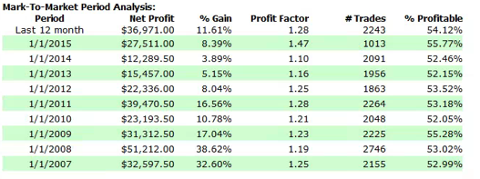
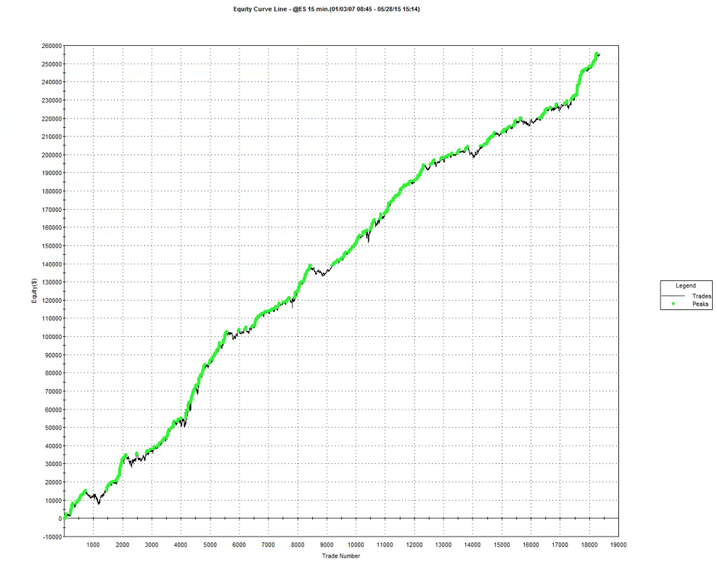
Let’s contrast the futures strategy with an example of a similar HFT strategy in equities.  Under the optimistic fill assumption the equity curve looks as follows:

Fig5

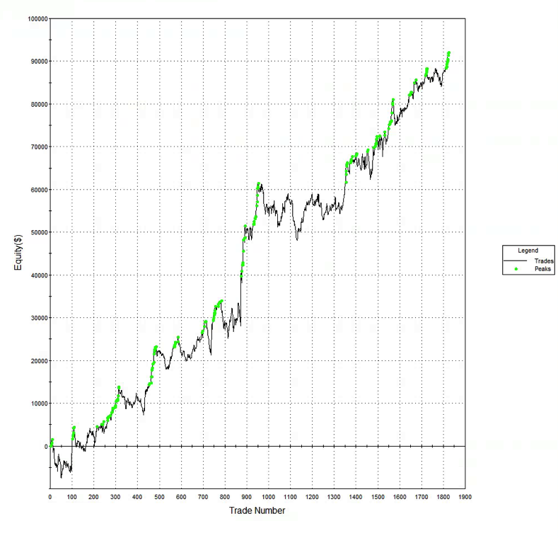
Under the more conservative fill assumption, the equity curve is obviously worse, but the strategy continues to produce excellent returns.  In other words, even if the market moves against the system on every single order, trading higher after a sell order is filled, or lower after a buy order is filled, the strategy continues to make money.

Fig6

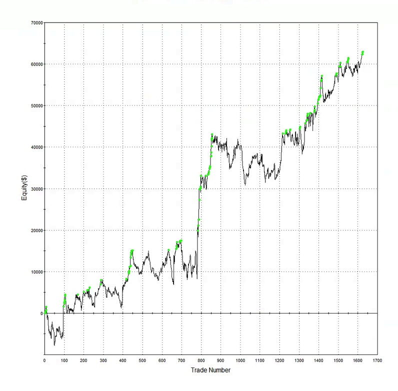
Market Microstructure

There is a fundamental reason for the discrepancy in the behavior of the two strategies under different fill scenarios, which relates to the very different microstructure of futures vs. equity markets.   In the case of the E-mini strategy the average trade might be, say, $50, which is equivalent to only 4 ticks (each tick is worth $12.50).  So the average trade: tick size ratio is around 4:1, at best.  In an equity strategy with similar average trade the tick size might be as little as 1 cent.  For a futures strategy, crossing the spread to enter or exit a trade more than a handful of times (or missing several limit order entries or exits) will quickly eviscerate the profitability of the system.  A HFT system in equities, by contrast, will typically prove more robust, because of the smaller tick size.

Of course, there are many other challenges to high frequency equity trading that futures do not suffer from, such as the multiplicity of trading destinations.  This means that, for instance, in a consolidated market data feed your system is likely to see trading opportunities that simply won’t arise in practice due to latency effects in the feed.  So the profitability of HFT equity strategies is often overstated, when measured using a consolidated feed.  Futures, which are traded on a single exchange, don’t suffer from such difficulties.  And there are a host of other differences in the microstructure of futures vs equity markets that the analyst must take account of.  But, all that understood, in general I would counsel that equities make an easier starting point for HFT system development, compared to futures.

Reflections on Careers in Quantitative Finance

CMU’s MSCF Program

Carnegie Mellon’s Steve Shreve is out with an interesting post on careers in quantitative finance, with his commentary on the changing landscape in quantitative research and the implications for financial education.

I taught at Carnegie Mellon in the late 1990’s, including its excellent Master’s program in quantitative finance that Steve co-founded, with Sanjay Srivastava.  The program was revolutionary in many ways and was immediately successful and rapidly copied by rival graduate schools (I help to spread the word a little, at Cambridge).

Fig1The core of the program remains largely unchanged over the last 20 years, featuring Steve’s excellent foundation course in stochastic calculus;  but I am happy to see that the school has added many, new and highly relevant topics to the second year syllabus, including market microstructure, machine learning, algorithmic trading and statistical arbitrage.  This has moved the program in terms of its primary focus, which was originally financial engineering, to include coverage of subjects that are highly relevant to quantitative investment research and trading.

It was this combination of sound theoretical grounding with practitioner-oriented training that made the program so successful.  As I recall, every single graduate was successful in finding a job on Wall Street, often at salaries in excess of $200,000, a considerable sum in those days.  One of the key features of the program was that it combined theoretical concepts with practical training, using a simulated trading floor gifted by Thomson Reuters (a model later adopted btrading-floor-1y the ICMA centre at the University of Reading in the UK).  This enabled us to test students’ understanding of what they had been taught, using market simulation models that relied upon key theoretical ideas covered in the program.  The constant reinforcement of the theoretical with the practical made for a much deeper learning experience for most students and greatly facilitated their transition to Wall Street.

Masters in High Frequency Finance

While CMU’s program has certainly evolved and remains highly relevant to the recruitment needs of Wall Street firms, I still believe there is an opportunity for a program focused exclusively on high frequency finance, as previously described in this post.  The MHFF program would be more computer science oriented, with less emphasis placed on financial engineering topics.  So, for instance, students would learn about trading hardware and infrastructure, the principles of efficient algorithm design, as well as HFT trading techniques such as order layering and priority management.  The program would also cover HFT strategies such as latency arbitrage, market making, and statistical arbitrage.  Students would learn both lower level (C++, Java) and higher level (Matlab, R) programming languages and there is  a good case for a mandatory machine code programming course also.  Other core courses might include stochastic calculus and market microstructure.

Who would run such a program?  The ideal school would have a reputation for excellent in both finance and computer science. CMU is an obvious candidate, as is MIT, but there are many other excellent possibilities.

Careers

I’ve been involved in quantitative finance since the beginning:  I recall programming one of the first 68000 Assembler microcomputers in the 1980s, which was ultimately used for an F/X system at a major UK bank. The ensuing rapid proliferation of quantitative techniques in finance has been fueled by the ubiquity of cheap computing power, facilitating the deployment of quantitate techniques that would previously been impractical to implement due to their complexity.  A good example is the machine learning techniques that now pervade large swathes of the finance arena, from credit scoring to HFT trading.  When I first began working in that field in the early 2000’s it was necessary to assemble a fairly sizable cluster of cpus to handle the computation load. These days you can access comparable levels of computational power on a single server and, if you need more, you can easily scale up via Azure or EC2.

fig3It is this explosive growth in computing power  that has driven the development of quantitative finance in both the financial engineering and quantitative investment disciplines. As the same time, the huge reduction in the cost of computing power has leveled the playing field and lowered barriers to entry.  What was once the exclusive preserve of the sell-side has now become readily available to many buy-side firms.  As a consequence, much of the growth in employment opportunities in quantitative finance over the last 20 years has been on the buy-side, with the arrival of quantitative hedge funds and proprietary trading firms, including my own, Systematic Strategies.  This trend has a long way to play out so that, when also taking into consideration the increasing restrictions that sell-side firms face in terms of their proprietary trading activity, I am inclined to believe that the buy-side will offer the best employment opportunities for quantitative financiers over the next decade.

It was often said that hedge fund managers are typically in their 30’s or 40’s when they make the move to the buy-side. That has changed in the last 15 years, again driven by the developments in technology.  These days you are more likely to find the critically important technical skills in younger candidates, in their late 20’s or early 30’s.  My advice to those looking for a career in quantitative finance, who are unable to find the right job opportunity, would be: do what every other young person in Silicon Valley is doing:  join a startup, or start one yourself.


High Frequency Trading Strategies

Most investors have probably never seen the P&L of a high frequency trading strategy.  There is a reason for that, of course:  given the typical performance characteristics of a HFT strategy, a trading firm has little need for outside capital.  Besides, HFT strategies can be capacity constrained, a major consideration for institutional investors.  So it is amusing to see the reaction of an investor on encountering the track record of a HFT strategy for the first time.  Accustomed as they are to seeing Sharpe ratios in the range of 0.5-1.5, or perhaps as high as 1.8, if they are lucky, the staggering risk-adjusted returns of a HFT strategy, which often have double-digit Sharpe ratios, are truly mind-boggling.

By way of illustration I have attached below the performance record of one such HFT strategy, which trades around 100 times a day in the eMini S&P 500 contract (including the overnight session).  Note that the edge is not that great – averaging 55% profitable trades and profit per contract of around half a tick – these are some of the defining characteristics of HFT trading strategies.  But due to the large number of trades it results in very substantial profits.  At this frequency, trading commissions are very low, typically under $0.1 per contract, compared to $1 – $2 per contract for a retail trader (in fact an HFT firm would typically own or lease exchange seats to minimize such costs).

Fig 2 Fig 3 Fig 4


Hidden from view in the above analysis are the overhead costs associated with implementing such a strategy: the market data feed, execution platform and connectivity capable of handling huge volumes of messages, as well as algo logic to monitor microstructure signals and manage order-book priority.  Without these, the strategy would be impossible to implement profitably.

SSALGOTRADING AD

Scaling things back a little, lets take a look at a day-trading strategy that trades only around 10 times a day, on 15-minute bars.  Although not ultra-high frequency, the strategy nonetheless is sufficiently high frequency to be very latency sensitive. In other words, you would not want to try to implement such a strategy without a high quality market data feed and low-latency trading platform capable of executing at the 1-millisecond level.  It might just be possible to implement a strategy of this kind using TT’s ADL platform, for example.

While the win rate and profit factor are similar to the first strategy, the lower trade frequency allows for a higher trade PL of just over 1 tick, while the equity curve is a lot less smooth reflecting a Sharpe ratio that is “only” around 2.7.

Fig 5 Fig 6 Fig 7


The critical assumption in any HFT strategy is the fill rate.  HFT strategies execute using limit or IOC orders and only a certain percentage of these will ever be filled.  Assuming there is alpha in the signal, the P&L grows in direct proportion to the number of trades, which in turn depends on the fill rate.  A fill rate of 10% to 20% is usually enough to guarantee profitability (depending on the quality of the signal). A low fill rate, such as would typically be seen if one attempted to trade on a retail trading platform, would  destroy the profitability of any HFT strategy.

To illustrate this point, we can take a look at the outcome if the above strategy was implemented on a trading platform which resulted in orders being filled only when the market trades through the limit price.  It isn’t a pretty sight.


Fig 8

The moral of the story is:  developing a HFT trading algorithm that contains a viable alpha signal is only half the picture.  The trading infrastructure used to implement such a strategy is no less critical.  Which is why HFT firms spend tens, or hundreds of millions of dollars developing the best infrastructure they can afford.