A High Frequency Scalping Strategy on Collective2

Scalping vs. Market Making

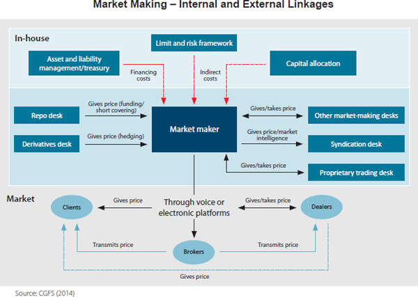
A market-making strategy is one in which the system continually quotes on the bid and offer and looks to make money from the bid-offer spread (and also, in the case of equities, rebates).  During a typical trading day, inventories will build up on the long or short side of the book as the market trades up and down.  There is no intent to take a market view as such, but most sophisticated market making strategies will use microstructure models to help decide whether to “lean” on the bid or offer at any given moment. Market makers may also shade their quotes to reduce the buildup of inventory, or even pull quotes altogether if they suspect that informed traders are trading against them (a situation referred to as “toxic flow”).  They can cover short positions through the repo desk and use derivatives to hedge out the risk of an accumulated inventory position.

marketmaking

A scalping strategy shares some of the characteristics of  a market making strategy:  it will typically be mean reverting, seeking to enter passively on the bid or offer and the average PL per trade is often in the region of a single tick.  But where a scalping strategy differs from market making is that it does take a view as to when to get long or short the market, although that view may change many times over the course of a trading session.  Consequently, a scalping strategy will only ever operate on one side of the market at a time, working the bid or offer; and it will typically never build inventory, since will it usually reverse and later try to sell for a profit the inventory it has previously purchased, hopefully at a lower price.

In terms of performance characteristics, a market making strategy will often have a double-digit Sharpe Ratio, which means that it may go for many days, weeks, or months, without taking a loss.  Scalping is inherently riskier, since it is taking directional bets, albeit over short time horizons.  With a Sharpe Ratio in the region of 3 to 5, a scalping strategy will often experience losing days and even losing months.

So why prefer scalping to market making?  It’s really a question of capability.  Competitive advantage in scalping derives from the successful exploitation of identified sources of alpha, whereas  market making depends primarily on speed and execution capability. Market making requires HFT infrastructure with latency measured in microseconds, the ability to layer orders up and down the book and manage order priority.  Scalping algos are generally much less demanding in terms of trading platform requirements: depending on the specifics of the system, they can be implemented successfully on many third party networks.

Developing HFT Futures Strategies

Some time ago my firm Systematic Strategies began research and development on a number of HFT strategies in futures markets.  Our primary focus has always been HFT equity strategies, so this was something of a departure for us, one that has entailed a significant technological obstacles (more on this in due course). Amongst the strategies we developed were several very profitable scalping algorithms in fixed income futures.  The majority trade at high frequency, with short holding periods measured in seconds or minutes, trading tens or even hundreds of times a day.
xtraderThe next challenge we faced was what to do with our research product.  As a proprietary trading firm our first instinct was to trade the strategies ourselves; but the original intent had been to develop strategies that could provide the basis of a hedge fund or CTA offering.  Many HFT strategies are unsuitable for that purpose, since the technical requirements exceed the capabilities of the great majority of standard trading platforms typically used by managed account investors. Besides, HFT strategies typically offer too limited capacity to be interesting to larger, institutional investors.

In the end we arrived at a compromise solution, keeping the highest frequency strategies in-house, while offering the lower frequency strategies to outside investors. This enabled us to keep the limited capacity of the highest frequency strategies for our own trading, while offering investors significant capacity in strategies that trade at lower frequencies, but still with very high performance characteristics.

HFT Bond Scalping

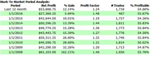
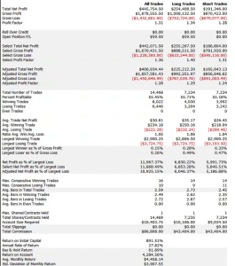
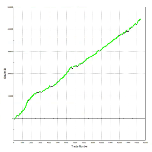
A typical example is the following scalping strategy in US Bond Futures.  The strategy combines two of the lower frequency algorithms we developed for bond futures that scalp around 10 times per session.  The strategy attempts to take around 8 ticks out of the market on each trade and averages around 1 tick per trade.   With a Sharpe Ratio of over 3, the strategy has produced net profits of approximately $50,000 per contract per year, since 2008.    A pleasing characteristic of this and other scalping strategies is their consistency:  There have been only 10 losing months since January 2008, the last being a loss of $7,100 in Dec 2015 (the prior loss being $472 in July 2013!)

Annual P&L

Fig2

Strategy Performance

fig4Fig3


Offering The Strategy to Investors on Collective2

The next challenge for us to solve was how best to introduce the program to potential investors.  Systematic Strategies is not a CTA and our investors are typically interested in equity strategies.  It takes a great deal of hard work to persuade investors that we are able to transfer our expertise in equity markets to the very different world of futures trading. While those efforts are continuing with my colleagues in Chicago, I decided to conduct an experiment:  what if we were to offer a scalping strategy through an online service like Collective2?  For those who are unfamiliar, Collective2 is an automated trading-system platform that allowed the tracking, verification, and auto-trading of multiple systems.  The platform keeps track of the system profit and loss, margin requirements, and performance statistics.  It then allows investors to follow the system in live trading, entering the system’s trading signals either manually or automatically.

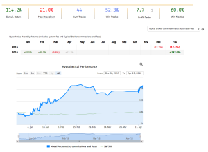
Offering a scalping strategy on a platform like this certainly creates visibility (and a credible track record) with investors; but it also poses new challenges.  For example, the platform assumes trading cost of around $14 per round turn, which is at least 2x more expensive than most retail platforms and perhaps 3x-5x more expensive than the cost a HFT firm might pay.  For most scalping strategies that are designed to take a tick out of the market such high fees would eviscerate the returns.  This motivated our choice of US Bond Futures, since the tick size and average trade are sufficiently large to overcome even this level of trading friction.  After a couple of false starts, during which we played around with the algorithms and boosted strategy profitability with a couple of low frequency trades, the system is now happily humming along and demonstrating the kind of performance it should (see below).

For those who are interested in following the strategy’s performance, the link on collective2 is here.


Collective2Perf

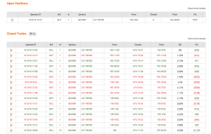
trades

Disclaimer

About the results you see on this Web site

Past results are not necessarily indicative of future results.

These results are based on simulated or hypothetical performance results that have certain inherent limitations. Unlike the results shown in an actual performance record, these results do not represent actual trading. Also, because these trades have not actually been executed, these results may have under-or over-compensated for the impact, if any, of certain market factors, such as lack of liquidity. Simulated or hypothetical trading programs in general are also subject to the fact that they are designed with the benefit of hindsight. No representation is being made that any account will or is likely to achieve profits or losses similar to these being shown.

In addition, hypothetical trading does not involve financial risk, and no hypothetical trading record can completely account for the impact of financial risk in actual trading. For example, the ability to withstand losses or to adhere to a particular trading program in spite of trading losses are material points which can also adversely affect actual trading results. There are numerous other factors related to the markets in general or to the implementation of any specific trading program, which cannot be fully accounted for in the preparation of hypothetical performance results and all of which can adversely affect actual trading results.

Material assumptions and methods used when calculating results

The following are material assumptions used when calculating any hypothetical monthly results that appear on our web site.

  • Profits are reinvested. We assume profits (when there are profits) are reinvested in the trading strategy.
  • Starting investment size. For any trading strategy on our site, hypothetical results are based on the assumption that you invested the starting amount shown on the strategy’s performance chart. In some cases, nominal dollar amounts on the equity chart have been re-scaled downward to make current go-forward trading sizes more manageable. In these cases, it may not have been possible to trade the strategy historically at the equity levels shown on the chart, and a higher minimum capital was required in the past.
  • All fees are included. When calculating cumulative returns, we try to estimate and include all the fees a typical trader incurs when AutoTrading using AutoTrade technology. This includes the subscription cost of the strategy, plus any per-trade AutoTrade fees, plus estimated broker commissions if any.
  • “Max Drawdown” Calculation Method. We calculate the Max Drawdown statistic as follows. Our computer software looks at the equity chart of the system in question and finds the largest percentage amount that the equity chart ever declines from a local “peak” to a subsequent point in time (thus this is formally called “Maximum Peak to Valley Drawdown.”) While this is useful information when evaluating trading systems, you should keep in mind that past performance does not guarantee future results. Therefore, future drawdowns may be larger than the historical maximum drawdowns you see here.

Trading is risky

There is a substantial risk of loss in futures and forex trading. Online trading of stocks and options is extremely risky. Assume you will lose money. Don’t trade with money you cannot afford to lose.

A High Frequency Market Making Algorithm


This algorithm builds on the research by Stoikova and Avelleneda in their 2009 paper “High Frequency Trading in a Limit Order Book“, 2009 and extends the basic algorithm in several ways:

  1. The algorithm makes two sided markets in a specified list of equities, with model parameters set at levels appropriate for each product.
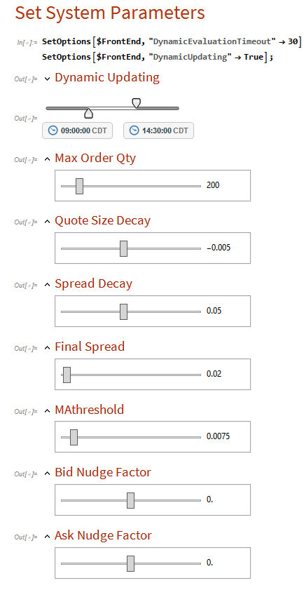
  2. The algorithm introduces an automatic mechanism for managing inventory, reducing the risk of adverse selection by changing the rate of inventory accumulation dynamically.
  3. The algorithm dynamically adjusts the range of the bid-ask spread as the trading session progresses, with the aim of minimizing inventory levels on market close.
  4. The extended algorithm makes use of estimates of recent market trends and adjusts the bid-offer spread to lean in the direction of the trend.
  5. A manual adjustment factor allows the market-maker to nudge the algorithm in the direction of reducing inventory.

The algorithm is implemented in Mathematica, and can be compiled to create dlls callable from with a C++ or Python application.

The application makes use of the MATH-TWS library to connect to the Interactive Brokers TWS or Gateway platform via the C++ api. MATH-TWS is used to create orders, manage positions and track account balances & P&L.


Day Trading System in VIX Futures – JonathanKinlay.com

This is a follow up to my earlier post on a Calendar Spread Strategy in VIX Futures (more information on calendar spreads ).

The strategy trades the front two months in the CFE VIX futures contract, generating an annual profit of around $25,000 per spread.

DAY TRADING SYSTEM
I built an equivalent day trading system in VIX futures in Trading Technologies visual ADL language, using 1-min bar data for 2010, and tested the system out-of-sample in 2011-2014. (for more information on X-Trader/ ADL go here).

The annual net PL is around $20,000 per spread, with a win rate of 67%.   On the downside, the profit factor is rather low and the average trade is barely 1/10 of a tick). Note that this is net of Bid-Ask spread of 0.05 ($50) and commission/transaction costs of $20 per round turn.  These cost assumptions are reasonable for online trading at many brokerage firms.

SSALGOTRADING AD

However, the strategy requires you to work the spread to enter passively (thereby reducing the cost of entry).  This is usually only feasible on a  platform suitable for a high frequency trading, where you can assume that your orders have acceptable priority in the limit order queue.  This will result in a reasonable proportion of your passive bids and offers will be executed.  Typically the spread trade is held throughout the session, exiting on close (since this is a day trading system).

Overall, while the trading system characteristics are reasonable, the spread strategy is better suited to longer (i.e. overnight) holding periods, since the VIX futures market is not the most liquid and the tick value is large.  We’ll take a look at other day trading strategies in more liquid products, like the S&P 500 e-mini futures, for example, in another post.

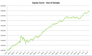
High Freq Strategy Equity Curve(click to enlarge)


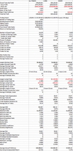
High Frequency Perf Results

(click to enlarge)

The Mathematics of Scalping

NOTE:  if you are unable to see the Mathematica models below, you can download the free Wolfram CDF player and you may also need this plug-in.

You can also download the complete Mathematica CDF file here.

In this post I want to explore aspects of scalping, a type of strategy widely utilized by high frequency trading firms.

I will define a scalping strategy as one in which we seek to take small profits by posting limit orders on alternate side of the book. Scalping, as I define it, is a strategy rather like market making, except that we “lean” on one side of the book. So, at any given time, we may have a long bias and so look to enter with a limit buy order. If this is filled, we will then look to exit with a subsequent limit sell order, taking a profit of a few ticks. Conversely, we may enter with a limit sell order and look to exit with a limit buy order.
The strategy relies on two critical factors:

(i) the alpha signal which tells us from moment to moment whether we should prefer to be long or short
(ii) the execution strategy, or “trade expression”

In this article I want to focus on the latter, making the assumption that we have some kind of alpha generation model already in place (more about this in later posts).

There are several means that a trader can use to enter a position. The simplest approach, the one we will be considering here, is simply to place a single limit order at or just outside the inside bid/ask prices – so in other words we will be looking to buy on the bid and sell on the ask (and hoping to earn the bid-ask spread, at least).

SSALGOTRADING AD

One of the problems with this approach is that it is highly latency sensitive. Limit orders join the limit order book at the back of the queue and slowly works their way towards the front, as earlier orders get filled. Buy the time the market gets around to your limit buy order, there may be no more sellers at that price. In that case the market trades away, a higher bid comes in and supersedes your order, and you don’t get filled. Conversely, yours may be one of the last orders to get filled, after which the market trades down to a lower bid and your position is immediately under water.

This simplistic model explains why latency is such a concern – you want to get as near to the front of the queue as you can, as quickly as possible. You do this by minimizing the time it takes to issue and order and get it into the limit order book. That entails both hardware (co-located servers, fiber-optic connections) and software optimization and typically also involves the use of Immediate or Cancel (IOC) orders. The use of IOC orders by HFT firms to gain order priority is highly controversial and is seen as gaming the system by traditional investors, who may end up paying higher prices as a result.

Another approach is to layer limit orders at price points up and down the order book, establishing priority long before the market trades there. Order layering is a highly complex execution strategy that brings addition complications.

Let’s confine ourselves to considering the single limit order, the type of order available to any trader using a standard retail platform.

As I have explained, we are assuming here that, at any point in time, you know whether you prefer to be long or short, and therefore whether you want to place a bid or an offer. The issue is, at what price do you place your order, and what do you do about limiting your risk? In other words, we are discussing profit targets and stop losses, which, of course, are all about risk and return.

Risk and Return in Scalping

Lets start by considering risk. The biggest risk to a scalper is that, once filled, the market goes against his position until he is obliged to trigger his stop loss. If he sets his stop loss too tight, he may be forced to exit positions that are initially unprofitable, but which would have recovered and shown a profit if he had not exited. Conversely,  if he sets the stop loss too loose, the risk reward ratio is very low – a single loss-making trade could eradicate the profit from a large number of smaller, profitable trades.

Now lets think about reward. If the trader is too ambitious in setting his profit target he may never get to realize the gains his position is showing – the market could reverse, leaving him with a loss on a position that was, initially, profitable. Conversely, if he sets the target too tight, the trader may give up too much potential in a winning trade to overcome the effects of the occasional, large loss.

It’s clear that these are critical concerns for a scalper: indeed the trade exit rules are just as important, or even more important, than the entry rules. So how should he proceed?

Theoretical Framework for Scalping

Let’s make the rather heroic assumption that market returns are Normally distributed (in fact, we know from empirical research that they are not – but this is a starting point, at least). And let’s assume for the moment that our trader has been filled on a limit buy order and is looking to decide where to place his profit target and stop loss limit orders. Given a current price of the underlying security of X, the scalper is seeking to determine the profit target of p ticks and the stop loss level of q ticks that will determine the prices at which he should post his limit orders to exit the trade. We can translate these into returns, as follows:

to the upside: Ru = Ln[X+p] – Ln[X]

and to the downside: Rd = Ln[X-q] – Ln[X]

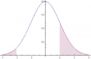
This situation is illustrated in the chart below.

Normal Distn Shaded

The profitable area is the shaded region on the RHS of the distribution. If the market trades at this price or higher, we will make money: p ticks, less trading fees and commissions, to be precise. Conversely we lose q ticks (plus commissions) if the market trades in the region shaded on the LHS of the distribution.

Under our assumptions, the probability of ending up in the RHS shaded region is:

probWin = 1 – NormalCDF(Ru, mu, sigma),

where mu and sigma are the mean and standard deviation of the distribution.

The probability of losing money, i.e. the shaded area in the LHS of the distribution, is given by:

probLoss = NormalCDF(Rd, mu, sigma),

where NormalCDF is the cumulative distribution function of the Gaussian distribution.

The expected profit from the trade is therefore:

Expected profit = p * probWin – q * probLoss

And the expected win rate, the proportion of profitable trades, is given by:

WinRate = probWin / (probWin + probLoss)

If we set a stretch profit target, then p will be large, and probWin, the shaded region on the RHS of the distribution, will be small, so our winRate will be low. Under this scenario we would have a low probability of a large gain. Conversely, if we set p to, say, 1 tick, and our stop loss q to, say, 20 ticks, the shaded region on the RHS will represent close to half of the probability density, while the shaded LHS will encompass only around 5%. Our win rate in that case would be of the order of 91%:

WinRate = 50% / (50% + 5%) = 91%

Under this scenario, we make frequent, small profits  and suffer the occasional large loss.

So the critical question is: how do we pick p and q, our profit target and stop loss?  Does it matter?  What should the decision depend on?

Modeling Scalping Strategies

We can begin to address these questions by noticing, as we have already seen, that there is a trade-off between the size of profit we are hoping to make, and the size of loss we are willing to tolerate, and the probability of that gain or loss arising.  Those probabilities in turn depend on the underlying probability distribution, assumed here to be Gaussian.

Now, the Normal or Gaussian distribution which determines the probabilities of winning or losing at different price levels has two parameters – the mean, mu, or drift of the returns process and sigma, its volatility.

Over short time intervals the effect of volatility outweigh any impact from drift by orders of magnitude.  The reason for this is simple:  volatility scales with the square root of time, while the drift scales linearly.  Over small time intervals, the drift becomes un-noticeably small, compared to the process volatility.  Hence we can assume that mu, the process mean is zero, without concern, and focus exclusively on sigma, the volatility.

What other factors do we need to consider?  Well there is a minimum price move, which might be 1 tick, and the dollar value of that tick, from which we can derive our upside and downside returns, Ru and Rd.  And, finally, we need to factor in commissions and exchange fees into our net trade P&L.

Here’s a simple formulation of the model, in which I am using the E-mini futures contract as an exemplar.

 WinRate[currentPrice_,annualVolatility_,BarSizeMins_, nTicksPT_, nTicksSL_,minMove_, tickValue_, costContract_]:=Module[{ nMinsPerDay, periodVolatility, tgtReturn, slReturn,tgtDollar, slDollar, probWin, probLoss, winRate, expWinDollar, expLossDollar, expProfit},
nMinsPerDay = 250*6.5*60;
periodVolatility = annualVolatility / Sqrt[nMinsPerDay/BarSizeMins];
tgtReturn=nTicksPT*minMove/currentPrice;tgtDollar = nTicksPT * tickValue;
slReturn = nTicksSL*minMove/currentPrice;
slDollar=nTicksSL*tickValue;
probWin=1-CDF[NormalDistribution[0, periodVolatility],tgtReturn];
probLoss=CDF[NormalDistribution[0, periodVolatility],slReturn];
winRate=probWin/(probWin+probLoss);
expWinDollar=tgtDollar*probWin;
expLossDollar=slDollar*probLoss;
expProfit=expWinDollar+expLossDollar-costContract;
{expProfit, winRate}]

For the ES contract we have a min price move of 0.25 and the tick value is $12.50.  Notice that we scale annual volatility to the size of the period we are trading (15 minute bars, in the following example).

Scenario Analysis

Let’s take a look at how the expected profit and win rate vary with the profit target and stop loss limits we set.  In the following interactive graphics, we can assess the impact of different levels of volatility on the outcome.

Expected Profit by Bar Size and Volatility

Expected Win Rate by Volatility

Notice to begin with that the win rate (and expected profit) are very far from being Normally distributed – not least because they change radically with volatility, which is itself time-varying.

For very low levels of volatility, around 5%, we appear to do best in terms of maximizing our expected P&L by setting a tight profit target of a couple of ticks, and a stop loss of around 10 ticks.  Our win rate is very high at these levels – around 90% or more.  In other words, at low levels of volatility, our aim should be to try to make a large number of small gains.

But as volatility increases to around 15%, it becomes evident that we need to increase our profit target, to around 10 or 11 ticks.  The distribution of the expected P&L suggests we have a couple of different strategy options: either we can set a larger stop loss, of around 30 ticks, or we can head in the other direction, and set a very low stop loss of perhaps just 1-2 ticks.  This later strategy is, in fact, the mirror image of our low-volatility strategy:  at higher levels of volatility, we are aiming to make occasional, large gains and we are willing to pay the price of sustaining repeated small stop-losses.  Our win rate, although still well above 50%, naturally declines.

As volatility rises still further, to 20% or 30%, or more, it becomes apparent that we really have no alternative but to aim for occasional large gains, by increasing our profit target and tightening stop loss limits.   Our win rate under this strategy scenario will be much lower – around 30% or less.

Non – Gaussian Model

Now let’s address the concern that asset returns are not typically distributed Normally. In particular, the empirical distribution of returns tends to have “fat tails”, i.e. the probability of an extreme event is much higher than in an equivalent Normal distribution.

A widely used model for fat-tailed distributions in the Extreme Value Distribution. This has pdf:

PDF[ExtremeValueDistribution[,],x]

 EVD

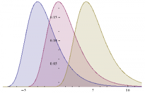
Plot[Evaluate@Table[PDF[ExtremeValueDistribution[,2],x],{,{-3,0,4}}],{x,-8,12},FillingAxis]

EVD pdf

Mean[ExtremeValueDistribution[,]]

+EulerGamma

Variance[ExtremeValueDistribution[,]]

EVD Variance

In order to set the parameters of the EVD, we need to arrange them so that the mean and variance match those of the equivalent Gaussian distribution with mean = 0 and standard deviation . hence:

EVD params

The code for a version of the model using the GED is given as follows

WinRateExtreme[currentPrice_,annualVolatility_,BarSizeMins_, nTicksPT_, nTicksSL_,minMove_, tickValue_, costContract_]:=Module[{ nMinsPerDay, periodVolatility, alpha, beta,tgtReturn, slReturn,tgtDollar, slDollar, probWin, probLoss, winRate, expWinDollar, expLossDollar, expProfit},
nMinsPerDay = 250*6.5*60;
periodVolatility = annualVolatility / Sqrt[nMinsPerDay/BarSizeMins];
beta = Sqrt[6]*periodVolatility / Pi;
alpha=-EulerGamma*beta;
tgtReturn=nTicksPT*minMove/currentPrice;tgtDollar = nTicksPT * tickValue;
slReturn = nTicksSL*minMove/currentPrice;
slDollar=nTicksSL*tickValue;
probWin=1-CDF[ExtremeValueDistribution[alpha, beta],tgtReturn];
probLoss=CDF[ExtremeValueDistribution[alpha, beta],slReturn];
winRate=probWin/(probWin+probLoss);
expWinDollar=tgtDollar*probWin;
expLossDollar=slDollar*probLoss;
expProfit=expWinDollar+expLossDollar-costContract;
{expProfit, winRate}]

WinRateExtreme[1900,0.05,15,2,30,0.25,12.50,3][[2]]

0.21759

We can now produce the same plots for the EVD version of the model that we plotted for the Gaussian versions :

Expected Profit by Bar Size and Volatility – Extreme Value Distribution

Expected Win Rate by Volatility – Extreme Value Distribution

Next we compare the Gaussian and EVD versions of the model, to gain an understanding of how the differing assumptions impact the expected Win Rate.

Expected Win Rate by Stop Loss and Profit Target

As you can see, for moderate levels of volatility, up to around 18 % annually, the expected Win Rate is actually higher if we assume an Extreme Value distribution of returns, rather than a Normal distribution.If we use a Normal distribution we will actually underestimate the Win Rate, if the actual return distribution is closer to Extreme Value.In other words, the assumption of a Gaussian distribution for returns is actually conservative.

Now, on the other hand, it is also the case that at higher levels of volatility the assumption of Normality will tend to over – estimate the expected Win Rate, if returns actually follow an extreme value distribution. But, as indicated before, for high levels of volatility we need to consider amending the scalping strategy very substantially. Either we need to reverse it, setting larger Profit Targets and tighter Stops, or we need to stop trading altogether, until volatility declines to normal levels.Many scalpers would prefer the second option, as the first alternative doesn’t strike them as being close enough to scalping to justify the name.If you take that approach, i.e.stop trying to scalp in periods when volatility is elevated, then the differences in estimated Win Rate resulting from alternative assumptions of return distribution are irrelevant.

If you only try to scalp when volatility is under, say, 20 % and you use a Gaussian distribution in your scalping model, you will only ever typically under – estimate your actual expected Win Rate.In other words, the assumption of Normality helps, not hurts, your strategy, by being conservative in its estimate of the expected Win Rate.

If, in the alternative, you want to trade the strategy regardless of the level of volatility, then by all means use something like an Extreme Value distribution in your model, as I have done here.That changes the estimates of expected Win Rate that the model produces, but it in no way changes the structure of the model, or invalidates it.It’ s just a different, arguably more realistic set of assumptions pertaining to situations of elevated volatility.

Monte-Carlo Simulation Analysis

Let’ s move on to do some simulation analysis so we can get an understanding of the distribution of the expected Win Rate and Avg Trade PL for our two alternative models. We begin by coding a generator that produces a sample of 1,000 trades and calculates the Avg Trade PL and Win Rate.

Gaussian Model

GenWinRate[currentPrice_,annualVolatility_,BarSizeMins_, nTicksPT_, nTicksSL_,minMove_, tickValue_, costContract_]:=Module[{ nMinsPerDay, periodVolatility, randObs, tgtReturn, slReturn,tgtDollar, slDollar, nWins,nLosses, perTradePL, probWin, probLoss, winRate, expWinDollar, expLossDollar, expProfit},
nMinsPerDay = 250*6.5*60;
periodVolatility = annualVolatility / Sqrt[nMinsPerDay/BarSizeMins];
tgtReturn=nTicksPT*minMove/currentPrice;tgtDollar = nTicksPT * tickValue;
slReturn = nTicksSL*minMove/currentPrice;
slDollar=nTicksSL*tickValue;
randObs=RandomVariate[NormalDistribution[0,periodVolatility],10^3];
nWins=Count[randObs,x_/;x>=tgtReturn];
nLosses=Count[randObs,x_/;xslReturn];
winRate=nWins/(nWins+nLosses)//N;
perTradePL=(nWins*tgtDollar+nLosses*slDollar)/(nWins+nLosses);{perTradePL,winRate}]

GenWinRate[1900,0.1,15,1,-24,0.25,12.50,3]

{7.69231,0.984615}

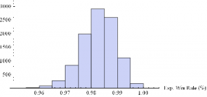
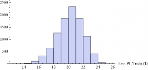
Now we can generate a random sample of 10, 000 simulation runs and plot a histogram of the Win Rates, using, for example, ES on 5-min bars, with a PT of 2 ticks and SL of – 20 ticks, assuming annual volatility of 15 %.

Histogram[Table[GenWinRate[1900,0.15,5,2,-20,0.25,12.50,3][[2]],{i,10000}],10,AxesLabel{“Exp. Win Rate (%)”}]

WinRateHist

Histogram[Table[GenWinRate[1900,0.15,5,2,-20,0.25,12.50,3][[1]],{i,10000}],10,AxesLabel{“Exp. PL/Trade ($)”}]

PLHist

Extreme Value Distribution Model

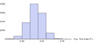
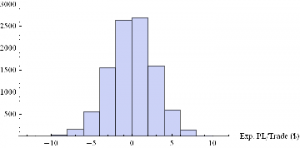
Next we can do the same for the Extreme Value Distribution version of the model.

GenWinRateExtreme[currentPrice_,annualVolatility_,BarSizeMins_, nTicksPT_, nTicksSL_,minMove_, tickValue_, costContract_]:=Module[{ nMinsPerDay, periodVolatility, randObs, tgtReturn, slReturn,tgtDollar, slDollar, alpha, beta,nWins,nLosses, perTradePL, probWin, probLoss, winRate, expWinDollar, expLossDollar, expProfit},
nMinsPerDay = 250*6.5*60;
periodVolatility = annualVolatility / Sqrt[nMinsPerDay/BarSizeMins];
beta = Sqrt[6]*periodVolatility / Pi;
alpha=-EulerGamma*beta;
tgtReturn=nTicksPT*minMove/currentPrice;tgtDollar = nTicksPT * tickValue;
slReturn = nTicksSL*minMove/currentPrice;
slDollar=nTicksSL*tickValue;
randObs=RandomVariate[ExtremeValueDistribution[alpha, beta],10^3];
nWins=Count[randObs,x_/;x>=tgtReturn];
nLosses=Count[randObs,x_/;xslReturn];
winRate=nWins/(nWins+nLosses)//N;
perTradePL=(nWins*tgtDollar+nLosses*slDollar)/(nWins+nLosses);{perTradePL,winRate}]

Histogram[Table[GenWinRateExtreme[1900,0.15,5,2,-10,0.25,12.50,3][[2]],{i,10000}],10,AxesLabel{“Exp. Win Rate (%)”}]

WinRateEVDHist

Histogram[Table[GenWinRateExtreme[1900,0.15,5,2,-10,0.25,12.50,3][[1]],{i,10000}],10,AxesLabel{“Exp. PL/Trade ($)”}]

PLEVDHist


Conclusions

The key conclusions from this analysis are:

  1. Scalping is essentially a volatility trade
  2. The setting of optimal profit targets are stop loss limits depend critically on the volatility of the underlying, and needs to be handled dynamically, depending on current levels of market volatility
  3. At low levels of volatility we should set tight profit targets and wide stop loss limits, looking to make a high percentage of small gains, of perhaps 2-3 ticks.
  4. As volatility rises, we need to reverse that position, setting more ambitious profit targets and tight stops, aiming for the occasional big win.