Matlab vs. Python

In a previous article I made a detailed comparison of Mathematica and Python and tried to identify areas where the former excels. Despite the many advantages of the Python technology stack, I was able to pinpoint a few areas in which I think Mathematica holds the upper hand. Whether those are sufficient to warrant the investment of time and money required to master the Wolfram Language is another matter, which the user must decide for himself.

In this comparison between Matlab and Python I won’t reiterate the strengths of the Python that make it the programming language of choice for so many developers. Let me instead focus on some of the key aspects of Matlab where I think the Mathworks product outshines its rival.

Matlab is designed for numerical computing, while Python is a general-purpose programming language that has become a major tool for scientific computing through libraries like NumPy, SciPy, and Matplotlib.

The key advantages of Matlab relative to Python, as I see them, are as follows:

Integrated Development Environment (IDE):

Matlab comes with a feature-rich IDE that is tailored for mathematical and engineering workflows. This includes tools for debugging, data visualization, GUI creation, and managing workspace variables. The Matlab IDE is specifically designed to streamline the development of mathematical and engineering applications.

Advanced Toolboxes:

Matlab offers a wide range of specialized toolboxes for different applications, including signal processing, control systems, neural networks, image processing, and many others. These toolboxes are professionally developed, rigorously tested, and regularly updated, providing a comprehensive suite of algorithms and functions for specific domains. With its vast ecosystem of scientific libraries Python has caught up with Matlab in recent years, and even overtaken it in some areas, but Matlab’s toolboxes are tried and battle-tested technologies that are used by millions of users in state-of-the-art applications.

Simulink:

Matlab provides Simulink, a platform for Model-Based Design for dynamic and embedded systems. Simulink is a graphical programming environment for modeling, simulating, and analyzing multidomain dynamical systems. This is particularly useful in engineering applications where system modeling and simulation are crucial.

Built-in Support for Matrix Operations:

Matlab (Matrix Laboratory) has inherent support for matrix operations and linear algebra, making it highly efficient for tasks that involve complex mathematical computations.

Performance:

Matlab is optimized for operations involving matrices and vectors, which are central to engineering and scientific computations. For certain numerical tasks, Matlab’s performance is superior due to its highly optimized code and ability to handle parallel computing and GPU acceleration effectively.

Matlab’s speed has further accelerated over the last decade due to just-in-time compilation. This feature automatically compiles Matlab’s interpreted code into machine code at runtime, which speeds up execution, especially in loops and computationally intensive tasks. The JIT compilation process is entirely transparent to the user, requiring no modifications to the code or the development process.
Python itself is an interpreted language and does not include JIT compilation in its standard implementation (CPython). However, JIT compilation can be introduced through third-party libraries or alternative Python implementations, such as Numba or PyPy.

Testing and Debugging:

Both Matlab and Python are equipped with robust testing and debugging tools that cater to their specific user bases. Matlab’s tools are tightly integrated into its IDE and are particularly tailored for numerical computing and engineering tasks. I would regard them as the industry standard in terms of features, ease of use and helpfulness. In contrast, Python’s testing and debugging ecosystem is more diverse, with multiple options available for different tasks, including third-party libraries that extend its capabilities.

Documentation and Support:

Matlab’s documentation is extensive, well-organized, and includes examples for a wide range of functions and toolboxes. Additionally, MathWorks provides excellent support services, including technical support and community forums, which can be particularly valuable for complex or specialized projects.

Conclusion

While Python has gained significant popularity in scientific computing, data science, and machine learning due to its open-source nature and the vast ecosystem of libraries, Matlab holds strong advantages in numerical computing, engineering applications, and when integrated solutions with robust support and documentation are required.

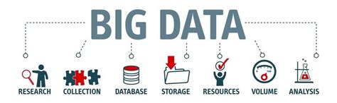
However, Python offers greater flexibility, scalability and has grown significantly in scientific computing. MATLAB historically had limitations with very large datasets, but recent releases have added features to improve performance with big data. Still, Python likely retains an advantage for extreme scales. The choice depends on the specific use case – for small-scale numerical computing and modeling MATLAB provides an integrated optimized environment while Python excels in general-purpose programming and very large-scale data intensive applications. However, both continue to evolve impressive capabilities so the lines are blurring. Ultimately data scientists and engineers are best served by being proficient in both languages.

Python vs. Wolfram Language

Python vs. Wolfram Language

As an avid user of both Python and Wolfram Language for technical computing, I’m often asked how they compare. Python’s strengths as an open-source language are clear:

  • Ubiquity – With millions of users, Python has become ubiquitous across fields like data science, ML engineering, web development, and scientific research. This massive adoption fuels continuous enhancement of its tools.
  • Comprehensive capabilities – Python’s expansive ecosystem of 200,000+ libraries spans everything from numerical computing to web frameworks to industrial automation. It is a versatile, widely-supported language for building end-to-end applications.
  • Approachability – Python’s straightforward syntax, multitude of online resources, and abundance of machine learning libraries like TensorFlow and PyTorch make it highly accessible for new programmers and non-CS domain experts alike.
  • Interoperability – Python integrates smoothly with everything from SQL and NoSQL databases to enterprise IT environments and microcontrollers like Raspberry Pi. This flexibility enables diverse production deployments.


In summary, Python offers benefits in ubiquity, breadth, approachability, and seamless interoperability with external systems. Together, they show the value of domain-specific and general-purpose languages for tackling modern analytics and engineering challenges.

However, while Python is a versatile, open-source language popular among developers, the Wolfram Language offers some unique advantages:

Powerful Symbolic Capabilities

One of the most powerful aspects of the Wolfram Language is its unparalleled symbolic manipulation abilities for mathematical computation. Operations like symbolic integration, solving equations analytically, theorem proving, model simplification and more are built deeply into the language in a way no other programming language matches. Python can conduct numeric computation and data analysis well, but does not have this domain of symbolic capabilities natively.

For any usage involving abstract mathematical development, derivation of analytical results, or formal proofs, the symbolic nature of the Wolfram Language is a major differentiator.


Wolfram Notebooks

offer notable advantages over Jupyter notebooks in Python:

  • More visual appeal – The Wolfram notebooks produce beautifully typeset output and publication-ready visualizations by default, whereas Jupyter’s output is more basic.
  • Greater configurability – Wolfram’s notebooks allow extensive styling, templating, and customization of content for different applications. Jupyter also enables some configuration, but not to the same degree.
  • Tighter integration – The Wolfram notebooks leverage the language’s underlying functions and capabilities more fluidly since it’s one integrated environment. Jupyter interfaces well with Python but there is still some separation.
  • Interactivity – Wolfram notebooks support advanced interactivity through Manipulate/Animate and instant visual output.

    Overall, while Jupyter notebooks are hugely popular among Python developers and enable great functionality, Wolfram’s notebook solution stands out as more robust, customizable, and visually polished. The tight integration with the Wolfram Language and computational capabilities augments interactive analysis in a way Jupyter can’t match.

Integrated Knowledge and Data

The Wolfram Language stands out in providing an “integrated knowledge base” that spans from sophisticated algorithms to real-world data across domains. This includes vast curated datasets on topics from architecture to chemistry to finance that can readily feed models and analyses without additional wrangling.

Additionally, the entity store concept allows users to author their own object-based, customizable data repositories. Python’s classes are focused on methods rather than data and while Python offers strong libraries for storing and accessing data, Wolfram facilitates more zero-friction application of real-world knowledge and entity-oriented data storage out-of-the-box. For minimizing time manipulating data or searching for reference algorithms before modeling, Wolfram Language excels.

The entity store in particular enables a very natural object/entity-based programming style that can integrate smoothly with Wolfram’s class system and its underlying symbolic capabilities. This unique data representation system differentiation is a key strength (for example, see the Equities Entity Store).

Interactivity and Prototyping

The Wolfram Language excels in hands-on analysis and rapid iteration thanks to its line-by-line execution and built-in Manipulate/Animate functions for customizable graphics, animations and interactive simulations. Python does allow some interactivity in Jupyter notebooks, but does not match Wolfram’s capabilities for creating interactive visualizations on-the-fly. This makes Wolfram Language uniquely well-suited for highly iterative, prototyping tasks that involve visual output. If ease of exploration and fluid development is a priority, the Wolfram Language has clear strengths.

Seamless Parallelization

The Wolfram Language has seamless built-in parallelization capabilities that allow code to efficiently utilize multi-core systems without the developer needing to directly manage threads or processes. Python can achieve parallelism through libraries, but the developer bears responsibility for managing dependencies and avoiding conflicts. Similarly, the Wolfram Language directly interfaces with Nvidia GPUs out-of-the-box for high performance numerical code with minimal extra effort. Thus, for users focused on computational speedup, Wolfram simplifies parallelization and GPU integration in very useful ways.

Python libraries like TensorFlow and PyTorch do hide GPU complexities well for deep learning. But in general, achieving parallel execution in Python places a greater burden on the developer. Wolfram’s approach dramatically lowers the barriers to leveraging multiple cores and GPU power for everyday computations.

Sophisticated Visualization

Creating publication-quality, customized visualizations requires just lines of code in the Wolfram Language, thanks to the built-in graphics capabilities. While Python offers powerful visualization through add-on libraries like Matplotlib, Seaborn, Bokeh, and Plotly, Wolfram’s out-of-the-box solutions may provide greater ease of use. However, from low-level control to interactive web plots, Python’s visualization options are quite extensive despite requiring more setup. Ultimately, for rapid high-level plotting, Wolfram Language has advantageous default capabilities. But Python gives more flexibility and customization options through its ecosystem of graphic libraries.

In summary, while Python offers flexibility and a large user base – advantages in its own right – the Wolfram Language dramatically reduces lines of code and development time. By curating real-world data, algorithms, and visualization in one coherent language and platform, it streamlines and accelerates quantitative work for scientists, analysts, economists and more.

If you do significant data analysis or modeling, I encourage you to try the Wolfram Language and see the difference yourself. It’s been a gamechanger for my productivity.

Generating Synthetic Market Data

Why Synthetic Data?

Synthetic market data has great potential for applications in financial research. Examples include testing the risk characteristics of a trading book or investment portfolio, developing trading strategies using previously unseen data, or simulating high frequency trading activity in a limit order book. It provides an answer to the criticism of curve fitting that is routinely levelled at existing approaches that use the single, observed historical path followed by an asset to construct investment and risk models. Such models, critics argue, are usually over-fitted to the historical data and are consequently unlikely to prove robust, going forward.

What is required is a model of the underlying asset processes that can then be used to generate a large number of price paths for all of the constituents of an investment portfolio. This should provide a more realistic assessment of the range of possible behaviours of the portfolio under a wide variety of market conditions, including during tail events.

Existing Methodology

Current approaches to modelling asset processes are often rudimentary and fail to capture the interplay of market dynamics that impact the evolution of the process. So, for example, we might begin by modelling the process of asset returns using a Gaussian or Student-T distribution. This immediately runs into the issue of under-representing the “fat tails” of empirical asset distributions, where tail events occur much more frequently than standard distributions would suggest. We might move on consider using the empirical distribution itself, and this might be sufficient for some applications.

But in many cases we want to generate a sequence of returns, or perhaps a time series of Open/High/Low/Close prices for modelling purposes. This is a challenge that is at least an order of magnitude more difficult. We not only have to ensure that the returns and/or prices at each individual time step are consistent (e.g. that the High > Low, in the case of prices, for example), but also that the sequence of returns is representative of known characteristics of financial assets such as serial autocorrelation, cross correlation and volatility clustering. GARCH models serve reasonably well in this context, but, for example, fail to capture long memory effects, amongst other deficiencies.

Deep Learning Models

Generative Adversarial Networks have become ubiquitous in the generation of “deep fakes” – .synthesised images generated by deep learning models that are close to indistinguishable from the real thing, whether it be the image of a human face, or medical images such X-ray scans. In 2019 Jinsung Yoon, Daniel Jarrett, and Mihaela van der Schaar published a paper on Time-series Generative Adversarial Networks (“TimeGAN”) in Neural Information Processing Systems (link to paper here) , a deep learning model that can be used to generate synthetic time series data.

An important characteristic of time series data is that it extends regular tabular data in the third dimension (i.e time):

As the authors note:

“A good generative model for time-series data should preserve temporal dynamics, in the sense that new sequences respect the original relationships between variables across time. Existing methods that bring generative adversarial networks (GANs) into the sequential setting do not adequately attend to the temporal correlations unique to time-series data. At the same time, supervised models for sequence prediction – which allow finer control over network dynamics – are inherently deterministic.”

They continue:

“[TimeGAN is a] novel framework for generating realistic time-series data that combines the flexibility of the unsupervised paradigm with the control afforded by supervised training. Through a learned embedding space jointly optimized with both supervised and adversarial objectives, we encourage the network to adhere to the dynamics of the training data during sampling”.

This sounds very promising and indeed the authors claim that “Qualitatively and quantitatively, we find that the proposed framework consistently and significantly outperforms state-of-the-art benchmarks with respect to measures of similarity and predictive ability” for several different types of time series dataset, including stock data.

A Brief Interlude on Generative Adversarial Networks

In the GAN architecture we implement two models: one to generate artificial data and another to distinguish artificial from real data. For example, a GAN model to generate artificial images of handwritten numbers would look approximately like this:

There are many architectures to consider for building the discriminator and the generator. We could build a deep neural network or Convolutional Neural Network (CNN) as well as other options.

TimeGAN

In the context of time series we face not only the problem of matching the features of synthetic and real data sequences, but also calibrating the time dynamics of the underlying generation process. TimeGAN addresses these challenges by using an unsupervised adversarial loss on both real and synthetic sequences, coupled with a stepwise supervised loss using the original data as supervision, thereby explicitly encouraging the model to capture the stepwise conditional distributions in the data. This takes advantage of the fact that there is more information in the training data than simply whether each datum is real or synthetic; we can expressly learn from the transition dynamics from real sequences.

A further innovative feature of the TimeGAN model in the introduction of an embedding network to provide a reversible mapping between features and latent representations, thereby reducing the high-dimensionality of the adversarial learning space. This capitalizes on the fact the temporal dynamics of even complex systems are often driven by fewer and lower-dimensional factors of variation.

Importantly, the supervised loss is minimized by jointly training both the embedding and generator networks, such that the latent space not only serves to promote parameter efficiency—it is specifically conditioned to facilitate the generator in learning temporal relationships.

The figure below shows how the various components are arranged and how the information flows between them during training in TimeGAN.

Further details of the TimeGAN model can be found in the paper and in the accompanying GitHub repository, which is found here.

Evaluating the Performance of TimeGAN

The researchers test the TimeGAN methodology using several different datasets, such as daily stock data for the period 2004 to 2019 downloaded from Google, including as features the volume and high, low, opening, and closing prices.

The TimeGAN model is trained for 50,000 epochs with a batch size of 128, using a 24-period rolling window, which the authors found to be the optimal window size. The trained synthesizer produces samples comprising a (128 x 24 x 5) dataframe of price and volume data which can then be compared to the original stock series. It is worth noting that the starting prices of each 24-period window are generated independently, meaning that, for example, the opening price in one sample window might be 10x larger than in another window. This immediately indicates one of the drawbacks of the TimeGAN approach: i.e. that the window length of the generated data is fixed and it can be challenging to stitch windows together to create a longer synthetic series, given that the initial prices for each vary considerably from window to window.

The data visualization methods chosen by the authors to evaluate the performance of the synthetic series in reproducing the features of the original series is problematic, at least as far as stock data is concerned. Both TSNE and PCA plots of the real vs. synthetic data appear to indicate a very close match:

This illustrates how misleading it can be to rely on data visualization for inference purposes. For stock data, there are some very basic tests that should first be performed to ensure the consistency of the synthetic output. In particular, in each row of the window, the High should exceed the Open, Low and Close prices, with the Low price falling below the Open, High and Close prices.

In my experimentation I found that after training the model for 50,000 epochs, the synthetic data failed these basic tests in around 15% of the sample. Further training rounds up to 100,000 epochs reduced the error rate to only 5% and it should be possible to eliminate almost all of these basic data issues with further rounds of training.

However, another basic problem with the synthetic data rapidly becomes apparent: the period to period (in this case, daily) returns have a strong tendency to diminish over time, typically being an order of magnitude larger at the start of each window than towards the end. This pattern of behavior is bound to introduce spurious autocorrelation and volatility-decay effects that are nowhere to be found in the real data series.

Finally, the fixed, limited window size and the independence of each window sample of synthetic data make it impossible to account for important characteristics such as volatility clustering or long memory effects in any adequate way.

Taken together, these flaws render the synthetic stock data produced by TimeGAN significantly unrepresentative and highly unreliable for modelling purposes.

Conclusion

TimeGAN is an important innovation in the field of synthetic data generation, with particular relevance to time series data. However it has significant limitations that make its application to financial time series problematic, in regard to the fixed window length, inconsistencies in the price data and spurious autocorrelation in the returns of the synthetic series it generates.

DataScience| Handling Big Data

Handling Large Files in CSV format with NumPy and Pandas

One of the major challenges that users face when trying to do data science is how to handle big data. Leaving aside the important topic of database connectivity/functionality and the handling of data too large to fit in memory, my concern here is with the issue of how to handle large data files, which are often in csv format, but which are not too large to fit into available memory.

It is well known that, due to their generality, Mathematica’s Import and Export functions are horribly slow when handling large csv files. For example, writing out a list of 10 million 64-bit reals takes almost 5 minutes:

No alt text provided for this image

and reading is also unacceptably slow:

No alt text provided for this image

Performance results like these create the impression that Mathematica is suitable for handling only “toy” problems, rather than the kind of large and complex data challenges faced by data scientists in the real world.

Sure, you can speed this up with ReadLine, but not by much, after doing all the string processing. And while the mx binary file format speeds up data handling enormously, it doesn’t address the issue of how to get the data into the requisite file format, other than via the WL DumpSave function – in other words, the data already has to be in a Mathematica notebook in order to write an mx file.

With purely numerical data once way to address this by using non-proprietary binary file formats. For example, in Python we create a NumPy array and use the tofile() method to output the data in real64 binary format, in less then 2 seconds:

No alt text provided for this image

Then in Mathematica the read process is equally fast when processing a file of numerical data in binary format, around 50x faster than the time taken to process the same file in csv format:

No alt text provided for this image

The procedure is just as fast in the reverse direction, with binary data exports from Mathematica taking a fraction of the time required to process the same data in csv format (around 200x faster!):

No alt text provided for this image

And the data is extremely fast read back in Python using the numpy fromfile method:

No alt text provided for this image

This procedure is robust enough to accommodate missing data. For instance, let’s replace some of the values in our data array with np.nan values and export the file once again in binary format:

No alt text provided for this image

Reading the binary file into Mathematica, we find no reduction in speed, as the np.nan values are stored as decimals, which are replaced by the value Indeterminate in the imported Mathematica array:

No alt text provided for this image

So, for purely numerical data we have a fast and reliable procedure for transferring data between Python, R and Mathematica using binary format. This means that we can load very large csv files in Python, do some pre-processing in pandas and export the massaged data in binary format for further analysis in Mathematica, if required.

More Complex Data Structures: the HDF5 Format

A major step in the right direction has been achieved through the significant effort that WR has put into implementing the HDF5 binary file format standard in the Wolfram Language. This serves two purposes: firstly, it can speed up the storage and retrieval of large datasets, by orders of magnitudes (depending on the data type); secondly, unlike Wolfram’s proprietary mx file format, HDF5 is an open source format that can store large, complex & hierarchical datasets that are accessible via Python, R and MatLab, as well as other languages/platforms, including Mathematica. So, working with the same dataset as before, but using HDF5 format, we get an speed-up of around 500x on the file write and around 270x on the file read:

No alt text provided for this image

Another major benefit of working in binary format is the enormous saving in disk storage, compared to csv:

No alt text provided for this image

So it becomes feasible to envisage a workflow in which some pre-processing of a very large dataset in csv format takes place initially in e.g. Python Pandas, the results of which are exported to a HDF5 or binary format file for further processing in Mathematica.

This advance does a great deal to address some of the major concerns about using Mathematica for large data science projects. And I am not sure that users are necessarily aware of its significance, given all the hoopla over more glamorous features that tend to get all the attention in new version releases.