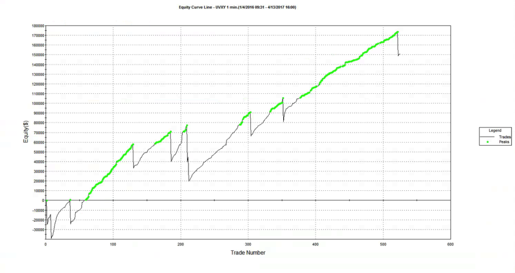
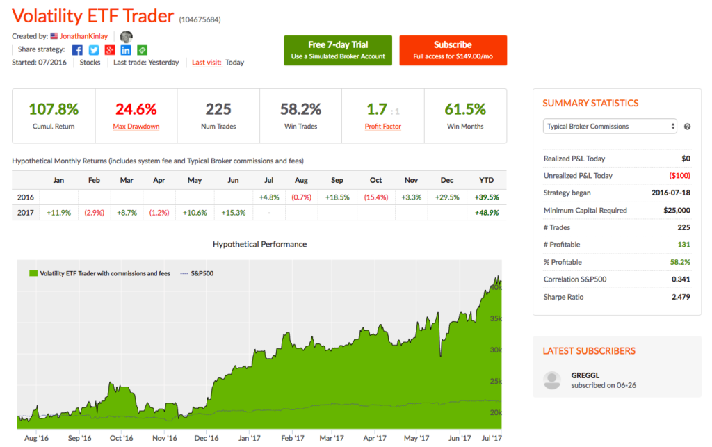
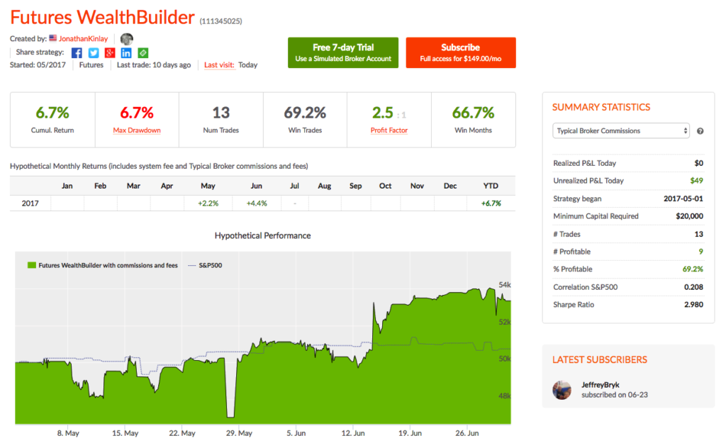
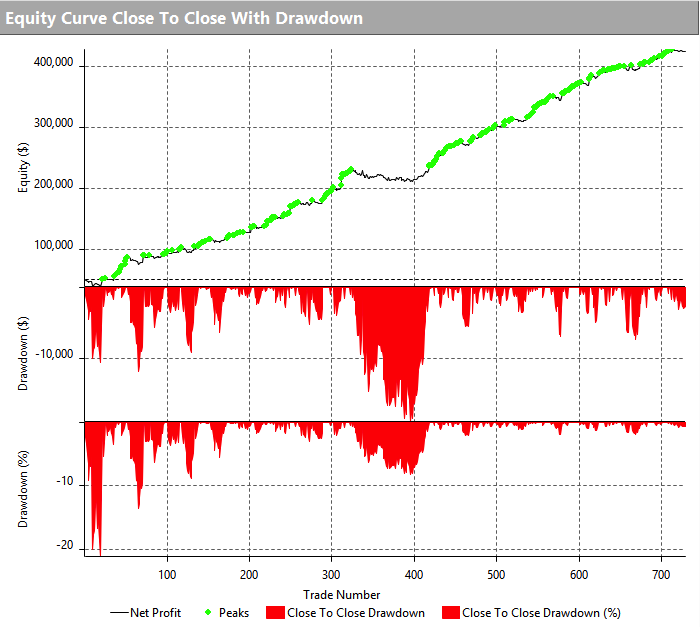
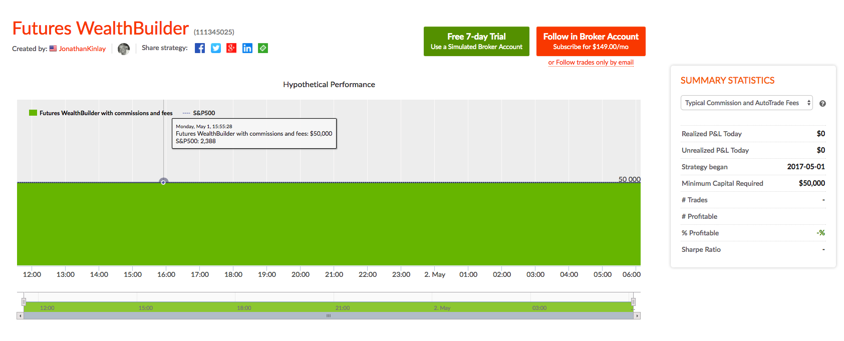
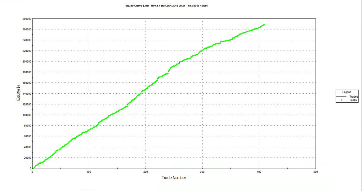
It isn’t often that you see an equity curve like the one shown below, which was produced by a systematic strategy built on 1-minute bars in the ProShares Ultra VIX Short-Term Futures ETF (UVXY):

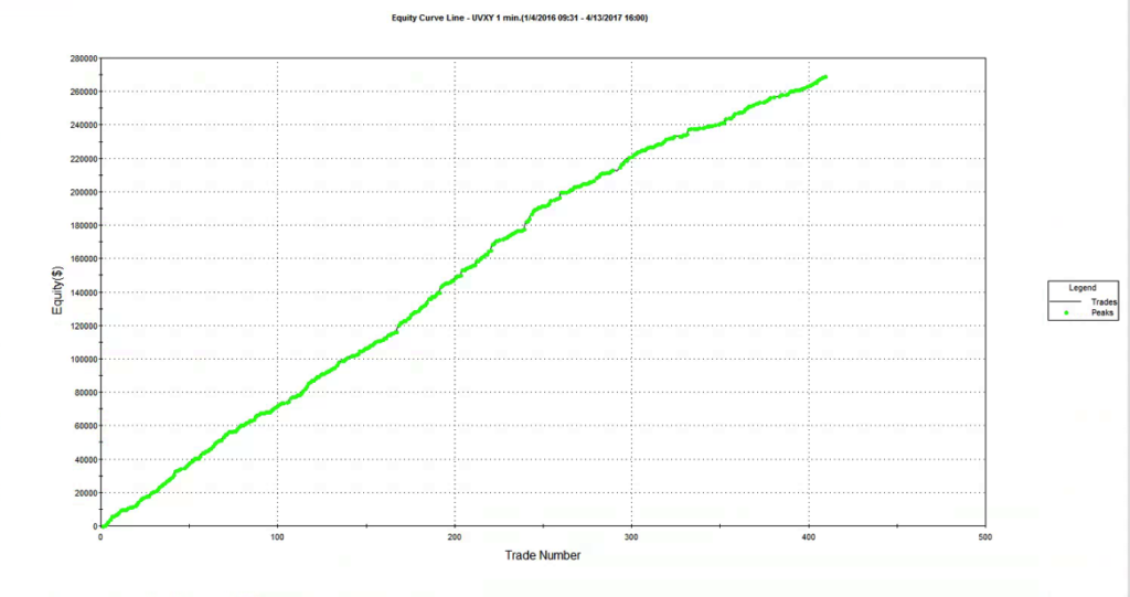
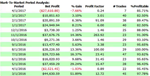
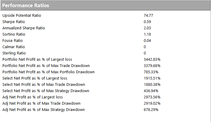
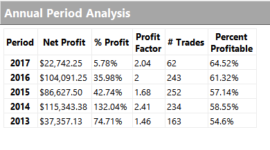
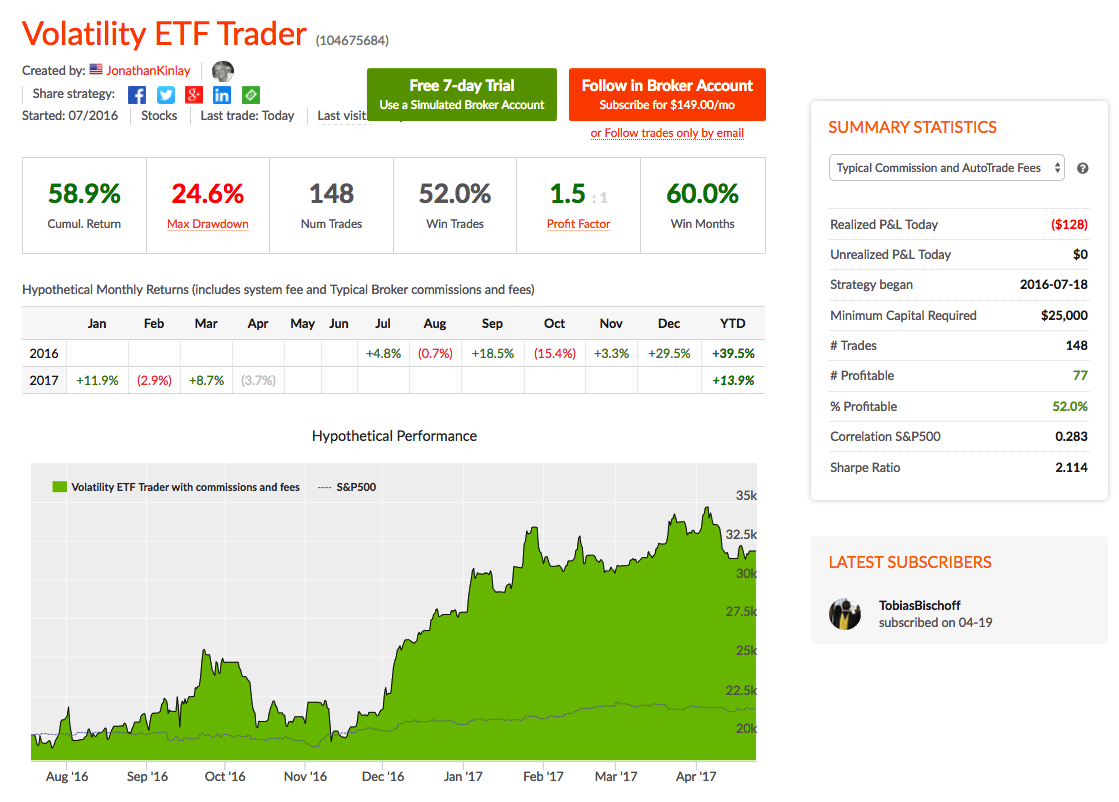
As the chart indicates, the strategy is very profitable, has a very high overall profit factor and a trade win rate in excess of 94%:

So, what’s not to like?  Well, arguably, one would like to see a strategy with a more balanced P&L, capable of producing profitable trades on the long as well as the short side. That would give some comfort that the strategy will continue to perform well regardless of whether the market tone is bullish or bearish. That said, it is understandable that the negative drift from carry in volatility futures, amplified by the leverage in the leveraged ETF product, makes it is much easier to make money by selling short.  This is  analogous to the long bias in the great majority of equity strategies, which relies on the positive drift in stocks.  My view would be that the short bias in the UVXY strategy is hardly a sufficient reason to overlook its many other very attractive features, any more than long bias is a reason to eschew equity strategies.

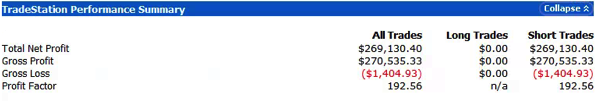
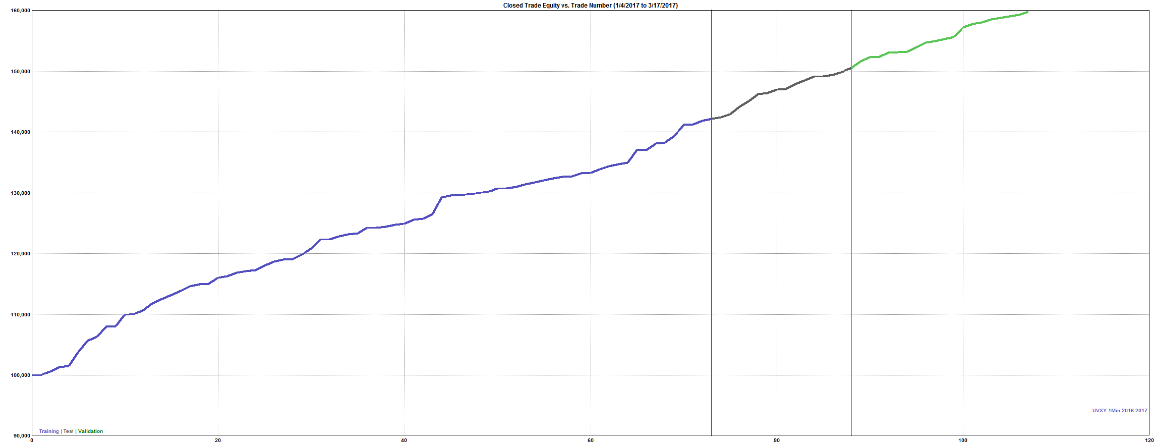
This example is similar to one we use in our training program for proprietary and hedge fund traders, to illustrate some of the pitfalls of strategy development.  We point out that the strategy performance has held up well out of sample – indeed, it matches the in-sample performance characteristics very closely.  When we ask trainees how they could test the strategy further, the suggestion is often made that we use Monte-Carlo simulation to evaluate the performance across a wider range of market scenarios than seen in the historical data.  We do this by introducing random fluctuations into the ETF prices, as well as in the strategy parameters, and by randomizing the start date of the test period.  The results are shown below. As you can see, while there is some variation in the strategy performance, even the worst simulated outcome appears very benign.

Around this point trainees, at least those inexperienced in trading system development, tend to run out of ideas about what else could be done to evaluate the strategy.  One or two will mention drawdown risk, but the straight-line equity curve indicates that this has not been a problem for the strategy in the past, while the results of simulation testing suggest that drawdowns are unlikely to be a significant concern, across a broad spectrum of market conditions.  Most trainees simply want to start trading the strategy as soon as possible (although the more cautious of them will suggest trading in simulation mode for a while).

As this point I sometimes offer to let trainees see the strategy code, on condition that they agree to trade the strategy with their own capital.   Being smart people, they realize something must be wrong, even if they are unable to pinpoint what the problem may be.  So the discussion moves on to focus in more detail the question of strategy risk.

A Deeper Dive into Strategy Risk

At this stage I point out to trainees that the equity curve shows the result from realized gains and losses. What it does not show are the fluctuations in equity that occurred before each trade was closed.

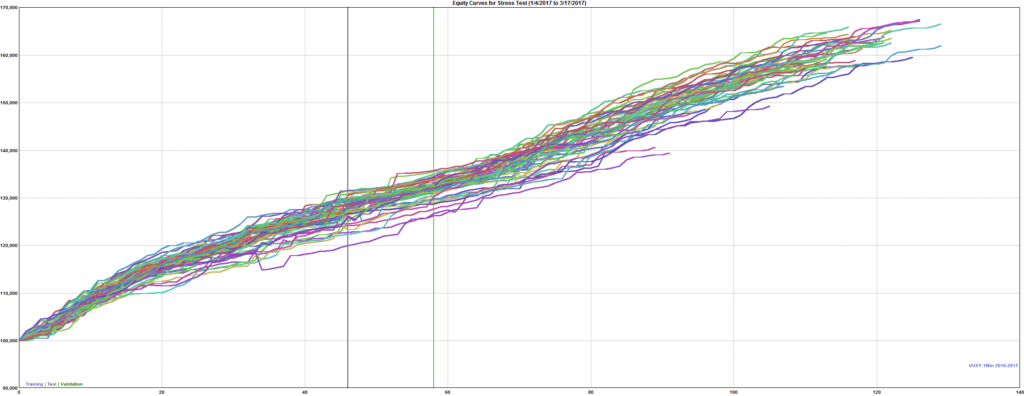
That information is revealed by the following report on the maximum adverse excursion (MAE), which plots the maximum drawdown in each trade vs. the final trade profit or loss.  Once trainees understand the report, the lights begin to come on.  We can see immediately that there were several trades which were underwater to the tune of $30,000, $50,000, or even $70,000 , or more, before eventually recovering to produce a profit.  In the most extreme case the trade was almost $80,000 underwater, before producing a profit of only a few hundred dollars. Furthermore, the drawdown period lasted for several weeks, which represents almost geological time for a strategy operating on 1-minute bars. It’s not hard to grasp the concept that risking $80,000 of your own money in order to make $250 is hardly an efficient use of capital, or an acceptable level of risk-reward.

Next, I ask for suggestions for how to tackle the problem of drawdown risk in the strategy.   Most trainees will suggest implementing a stop-loss strategy, similar to those employed by thousands of  trading firms.  Looking at the MAE chart, it appears that we can avert the worst outcomes with a stop loss limit of, say, $25,000.  However, when we implement a stop loss strategy at this level, here’s the outcome it produces:

Now we see the difficulty.  Firstly, what a stop-loss strategy does is simply crystallize the previously unrealized drawdown losses.  Consequently, the equity curve looks a great deal less attractive than it did before.  The second problem is more subtle: the conditions that produced the loss-making trades tend to continue for some time, perhaps as long as several days, or weeks.  So, a strategy that has a stop loss risk overlay will tend to exit the existing position, only to reinstate a similar position more or less immediately.  In other words, a stop loss achieves very little, other than to force the trader to accept losses that the strategy would have made up if it had been allowed to continue.  This outcome is a difficult one to accept, even in the face of the argument that a stop loss serves the purpose of protecting the trader (and his firm) from an even more catastrophic loss.  Because if the strategy tends to re-enter exactly the same position shortly after being stopped out, very little has been gained in terms of catastrophic risk management.

Luck and the Ethics of Strategy Design

What are the learning points from this exercise in trading system development?  Firstly, one should resist being beguiled by stellar-looking equity curves: they may disguise the true risk characteristics of the strategy, which can only be understood by a close study of strategy drawdowns and  trade MAE.  Secondly, a lesson that many risk managers could usefully take away is that a stop loss is often counter-productive, serving only to cement losses that the strategy would otherwise have recovered from.

A more subtle point is that a Geometric Brownian Motion process has a long-term probability of reaching any price level with certainty.  Accordingly, in theory one has only to wait long enough to recover from any loss, no matter how severe.   Of course, in the meantime, the accumulated losses might be enough to decimate the trading account, or even bring down the entire firm (e.g. Barings).  The point is,  it is not hard to design a system with a very seductive-looking backtest performance record.

If the solution is not a stop loss, how do we avoid scenarios like this one?  Firstly, if you are trading someone else’s money, one answer is: be lucky!  If you happened to start trading this strategy some time in 2016, you would probably be collecting a large bonus.  On the other hand, if you were unlucky enough to start trading in early 2017, you might be collecting a pink slip very soon.  Although unethical, when you are gambling with other people’s money, it makes economic sense to take such risks, because the potential upside gain is so much greater than the downside risk (for you). When you are risking with your own capital, however, the calculus is entirely different.  That is why we always trade strategies with our own capital before opening them to external investors (and why we insist that our prop traders do the same).

As a strategy designer, you know better, and should act accordingly.  Investors, who are relying on your skills and knowledge, can all too easily be seduced by the appearance of a strategy’s outstanding performance, overlooking the latent risks it hides.  We see this over and over again in option-selling strategies, which investors continue to pile into despite repeated demonstrations of their capital-destroying potential.  Incidentally, this is not a point about backtest vs. live trading performance:  the strategy illustrated here, as well as many option-selling strategies, are perfectly capable of producing live track records similar to those seen in backtest.  All you need is some luck and an uneventful period in which major drawdowns don’t arise.  At Systematic Strategies, our view is that the strategy designer is under an obligation to shield his investors from such latent risks, even if they may be unaware of them.  If you know that a strategy has such risk characteristics, you should avoid it, and design a better one.  The risk controls, including limitations on unrealized drawdowns (MAE) need to be baked into the strategy design from the outset, not fitted retrospectively (and often counter-productively, as we have seen here).

The acid test is this:  if you would not be prepared to risk your own capital in a strategy, don’t ask your investors to take the risk either.

The ethical principle of “do unto others as you would have them do unto you” applies no less in investment finance than it does in life.

Strategy Code