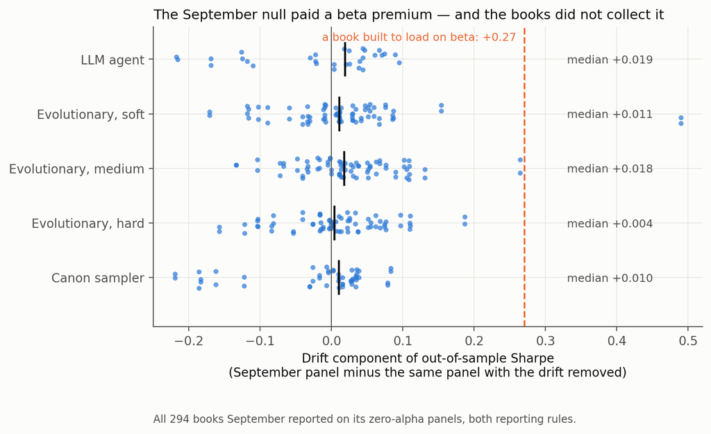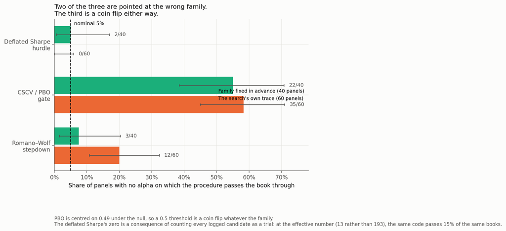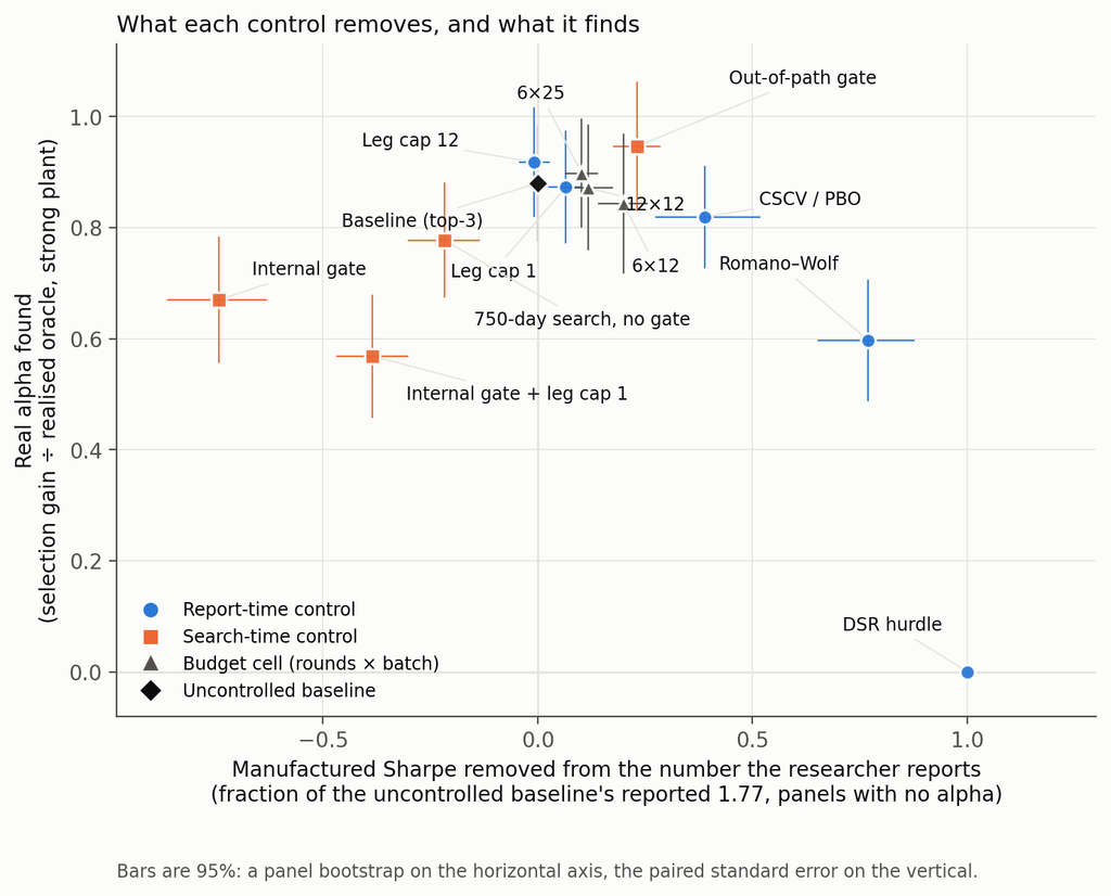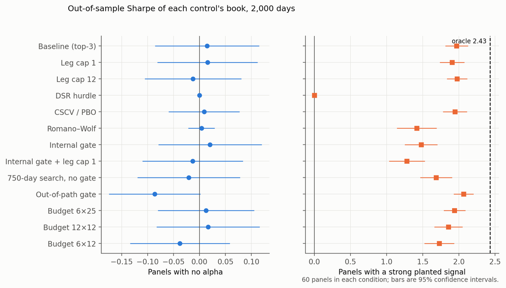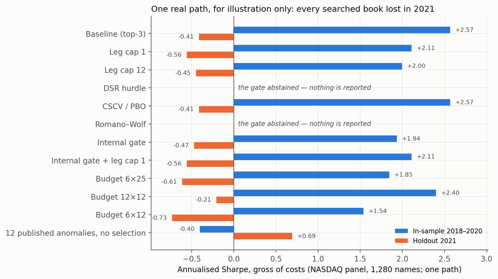

A Sharpe of 2.1 From Nothing: The Second Number Your Agent Doesn’t Log

September 2026

I gave a research agent four years of prices with no predictable structure in them — none, by construction — and it came back with a long/short book, an in-sample Sharpe of 2.1, and a paragraph explaining the economics of an effect that does not exist.

That is the measurement in this post. The more useful result is the second one: 88% of that number is accounted for by two integers — how many backtests the agent ran, and how many of the winners it blended into the book it reported. Only one of those is in the log everybody proposes to collect.

This closes a sequence. In August, having built an agentic research pipeline in May and measured a 2× lift in hypotheses tested per week, I priced a risk I had not thought to price: independent research runs against the same model produce books correlated at 0.62, a crowding exposure that appears in nobody’s risk report. That post ended with a claim I stated and did not measure — that faster hypothesis generation makes overfitting worse rather than better. This is the measurement, and my pre-registered prediction about how it would come out was wrong.


The one property agentic research has that human research never had

Every multiple-testing correction in finance founders on the same rock: you cannot observe the denominator. Harvey, Liu and Zhu built their t-statistic hurdle on an estimate of how many factors had been tried across the profession, not how many were published [1]. Harvey’s 2017 AFA presidential address is largely an argument about unreported trials [2]. The Deflated Sharpe Ratio requires you to supply the number of trials, and its authors are candid that in practice you are guessing [3]. Each method asks the researcher a question the researcher cannot honestly answer: how many things did you try before this one?

An agentic pipeline is different in exactly one respect. It has to ask the harness for every backtest it runs. The trial count is not a memory or an act of professional honesty. It is a log file.

So I built a minimal research agent, gave it one tool, recorded everything, and checked what the log is worth. The short answer is that it is worth less than I expected, for a reason that turns out to be measurable and fixable.


Setup

The harness. One command: submit up to 25 expressions, receive their in-sample scores. At most 12 such calls. The agent never sees prices, dates, tickers, or the holdout — the panel is anonymised to integer asset IDs and an integer time index, and the holdout files were physically absent from the filesystem while the runs executed. Every submission is logged with a timestamp, alongside a one-line hypothesis per batch and a free-text journal. The run ends when the agent reports exactly three signals.

What a “book” is, and the two counts that matter. Every arm’s output is scored the same way: three signals, equal-weighted into one book. The pre-registered primary rule takes the three highest-scoring signals a run evaluated, not the three it chose to report — the gap between the two is small and is itself reported below. N is the number of trials in the log. k is the number of additive legs in the resulting book: three for a searcher whose signals are single expressions, more for one whose signals are themselves sums. Those two integers carry the whole argument.

The signal language. A small price-only grammar: returns, moving averages, rolling moments, range position, rolling beta and correlation to the equal-weight panel, plus cross-sectional and time-series normalisations and arithmetic. It is the grammar from the August post, which matters — it was fixed before this hypothesis existed. Each signal becomes a dollar-neutral, rank-weighted long/short book with a one-day implementation lag.

The comparison arms. Three mechanical arms plus a no-selection placebo. The two that search run at the agent’s interaction schedule — 12 rounds of 25 candidates, feedback once per round. Matching rounds rather than evaluations is deliberate: in adaptive data analysis the damage scales with how many times you look and act, not with the raw query count [4].

ArmWhat it is
AGENTThe LLM researcher above
OPTEvolutionary search over the same grammar, at three selection pressures (soft, medium, hard — how aggressively each generation is bred from the current leaders)
CANON-SAMPLERCanon-shaped expressions with jittered parameters, no feedback — prior direction without optimisation
CANON placeboTwelve published anomalies in the same grammar, no selection at all

The data. The primary setting is synthetic: factor-structured panels with regime-switching volatility and fat tails, and zero predictability by construction. Volatility is forecastable; returns are not. The true Sharpe of every signal is zero, so every point of in-sample Sharpe is selection, and I can generate independent panels at will. The second setting is the real NASDAQ panel from the August post — 1,280 names, 2018–2023, train through 2021, holdout 2022 to May 2023.

The analysis plan, estimators, inclusion rule and predictions were committed to git before the first agent run. The repo holds the commit history, every harness log with its batch notes and research journals, a manifest of all 227 attempted runs including the five abandoned and why, and a list of every deviation from the plan.


1. What a research agent does with data that contains nothing

Twelve independent zero-alpha panels, one agent run each, identical prompt to the real-panel runs.

Every run found something. Every run wrote a confident rationale. From the report of a run on a panel whose returns are serially unpredictable by construction:

“All three combine the two independently validated engines: long-horizon cross-sectional mean reversion (ma 120-250, plateau confirmed across ret, ma, minr and maxr formulations at horizons 60-250) and a weekly return echo (returns from days t-8 to t-5 predict positively, with a coherent oscillating lag profile).”

There is no echo. There is no reversal. There is nothing.

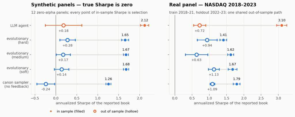
Zero-alpha panelsReported in-sample SharpeRealised out-of-sample Sharpe
LLM agent (12 runs)2.12 (SE 0.10)+0.18 (SE 0.44)
Evolutionary, soft (12 panels)1.68 (SE 0.07)+0.14 (SE 0.24)
Evolutionary, medium1.67 (SE 0.05)+0.17 (SE 0.22)
Evolutionary, hard1.65 (SE 0.11)+0.28 (SE 0.22)
Canon sampler, no feedback1.26 (SE 0.08)−0.24 (SE 0.29)

The reported book is the equal-weight composite of the three highest-scoring signals a run evaluated — the pre-registered primary rule, which is why it differs slightly from what the agent chose to report. True out-of-sample Sharpe is zero for every arm by construction, and every row is consistent with that. Standard errors are across panels.

A Sharpe ratio of 2.12, in-sample, on a book, over four years of daily data, from a panel with no signal in it.

A little over half of that is textbook. The expected maximum Sharpe of a single expression over the agent’s own median 146 logged trials is 1.15 (SE 0.03, across the twelve panels’ random-expression pools) — the expected-maximum-Sharpe effect [3], computed here as the exact order statistic over an empirical null pool drawn from the same grammar. That accounts for 54% of the 2.12. Note what the benchmark cannot do: those are single expressions, and it takes a single expression as the answer. Hold that thought — the missing 0.97 is the subject of section 3.

The agent’s own judgment is not the problem. It usually declines to report its top three by raw score, preferring what it calls “plateau” specifications; that restraint moves the number by 0.03 (2.08 chosen versus 2.12 argmax).

In-sample versus out-of-sample by search arm

2. It manufactures more than a machine built to overfit

Paired by panel, against the evolutionary optimiser at the identical interaction schedule, using only the twelve primary runs:

Contrast, in-sample Sharpe (12 paired panels)DifferenceSEt
Agent − evolutionary (soft)+0.440.11+3.9
Agent − evolutionary (medium)+0.450.11+4.1
Agent − evolutionary (hard)+0.460.09+5.2

On the real panel the gap is larger: 3.10 against 1.41–1.67.

That is the in-sample difference, and it is solid. The out-of-sample differences are not: those contrasts carry standard errors of 0.35 to 0.42, against a minimum detectable effect of about 1.0 Sharpe, and the pre-registered block bootstrap on the real panel returns a 95% interval of [−0.53, +1.99] for the agent’s realised Sharpe alone. Nothing in this study establishes that the agent’s books perform worse out of sample than a mechanical optimiser’s. What it establishes is that at a matched interaction budget, the agent converts noise into reported Sharpe more efficiently.

My pre-registered prediction was the opposite — that the model’s priors would act as a regulariser, keeping it in the published canon rather than in the noise, so it would overfit less. Wrong, at t ≈ 4.

3. Where the extra Sharpe comes from is not more searching

The mechanism is in the logs, and it is not model priors.

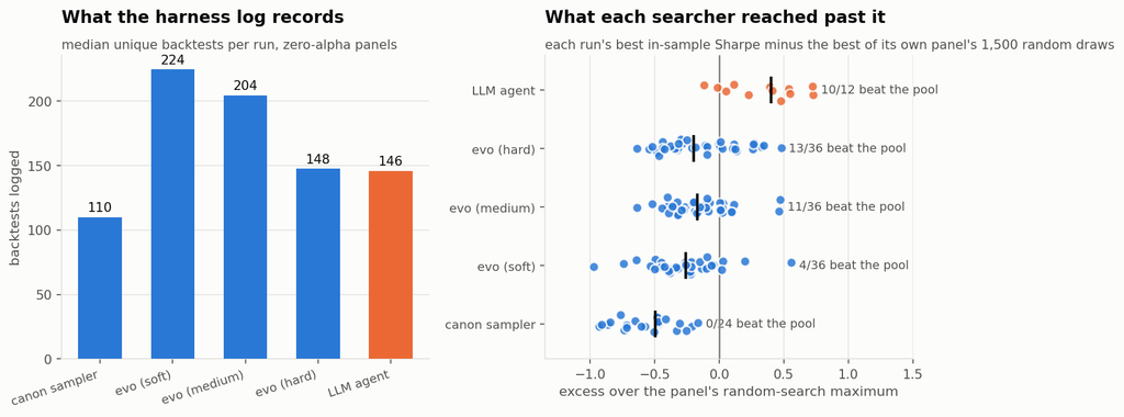
The agent logs a median of 146 unique backtests per zero-alpha run, against 148–225 for the evolutionary arms: level with the hardest setting, well below the softer ones. It is not searching harder — and note that the largest gap in the table above, +0.46, is against the arm that runs the same number of trials.

The difference is in what gets reported. Every run reports three signals, which are equal-weighted into one book. For the mechanical arms each of those three is a single expression, so the book has 3 legs. The agent’s three are themselves sums: a median of 4.2 legs each on zero-alpha panels, so its book carries about 12.5. That is the second integer, and no trial-count correction records it.

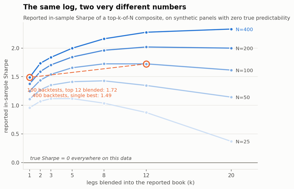
To isolate it I ran a controlled experiment on the zero-alpha panels with no agent involved: draw N random expressions, keep the top k by in-sample Sharpe, equal-weight them into a book, and record what the book reports.

The selection-plus-aggregation surface

Moving between curves is the familiar overfitting-versus-trials axis. Moving right along a curve is the aggregation axis nobody logs. The two trade off against each other: a pipeline that logs 100 backtests and blends its top 12 reports 1.72, while one that logs 400 and reports a single best reports 1.49. No alpha in either case, and the first pipeline’s log looks four times cleaner.

The arithmetic is standard portfolio algebra pointed at noise. Selecting k signals on in-sample performance and averaging them keeps the selected mean and cuts the variance — but the legs are not independent, so the gain is √(k / (1 + (k−1)ρ̄)), not √k. Fitting that form column by column over the monotone region gives ρ̄ of 0.41–0.47 at the trial counts that matter here, a ceiling of about 1.5× however many legs you add. That is why the curves flatten. They turn down at small N for a different reason: once k is a large fraction of N you are averaging in candidates that were barely selected at all. Novy-Marx made the combination point for strategies built from multiple signals and derived corrected critical values for it [5]; what is new here is an agent that was never asked to combine anything doing it unprompted, and the interchangeability of the two axes at a fixed log.

The closure. Take each run’s own logged trial count and its own book leg count, look up what blind top-k-of-N selection produces at that point on the surface, and compare:

ArmMedian trialsLegs in bookBlind top-k-of-N predictsActually reportedResidual
LLM agent14612.51.862.12+0.26
Evolutionary, hard14831.681.65−0.03
Evolutionary, medium20531.731.67−0.05
Evolutionary, soft22531.771.68−0.09
Canon sampler11031.561.26−0.31

Two integers and no model price the evolutionary arms to within 0.09, and account for 88% of the agent’s number. The residual is +0.26 (t ≈ 2.1 once the surface’s own estimation error is propagated) — small next to the 1.86 that blind selection explains. And the leg axis alone carries most of the agent’s edge over the mechanical searchers: holding trials at the agent’s own 146 and moving the book from 3 legs to 12.5 adds +0.25, against a measured agent-minus-mechanical gap of +0.45.

So the agent beats the optimiser and is beaten by blind selection at its own operating point, and both facts have one cause. It blends; they do not.

That also settles what happened to the estimator I pre-registered. I had planned to report an effective trial count — the random draws from this grammar needed to match a run’s best score. It cannot be computed for most agent runs: 10 of 12 exceed the best their own panel’s 1,500-draw random pool reached, so no trial count reproduces them. That is partly a property of a finite pool and it is not agent-specific — 13 of 36 hard evolutionary runs also clear their pool — so nothing here rests on it. The direction is informative, though: a deeper random-expression pool (depth 6, mean complexity 5.9 against the shallow pool’s 3.6) lifts the 99th percentile from 0.95 to 1.24 and the maximum to 1.79 without closing the gap, because random expressions almost never build composites — mean legs 1.15.

Depth is not the axis. Blending is.

What the log records versus what random search reaches

4. The real panel

Six agent runs on the NASDAQ panel, trained through 2021, scored on 2022 to May 2023.

Real panelTrainHoldoutLegs in bookDaily turnover
LLM agent (6)3.10 (SE 0.15)+0.72 (SE 0.18)6.00.24
Canon sampler (5)1.79 (SE 0.10)+1.09 (SE 0.07)30.45
Evolutionary, soft (5)1.67 (SE 0.13)+1.13 (SE 0.16)30.43
Evolutionary, medium (5)1.62 (SE 0.09)+0.63 (SE 0.32)30.26
Evolutionary, hard (5)1.41 (SE 0.10)+0.94 (SE 0.29)30.49
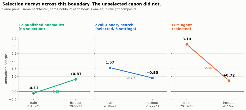
12 published anomalies, no selection−0.11+0.810.14

The last row is the control that makes the rest interpretable, and it is scored exactly like every other row — one equal-weight composite, same backtester, same holdout — with no selection applied. It does not decay across this boundary. It improves, from −0.11 to +0.81. The 2022–23 environment was kinder to these exposures on this universe than the training window was.

So the regime component of the agent’s decay is not merely small; it is negative. The control licenses one claim and not a stronger one: the unselected canon did not decay here, so the regime cannot explain the agent’s 2.4-point gap. It does not follow that selection explains all of it — the canon composite is loaded the opposite way from a book selected to score 3.10 in the training window, and the pre-registered random-search leg that would have measured the selection component directly was not run.

Note what the ordering does not do. It is not monotone — the medium evolutionary arm has the lowest holdout Sharpe of any arm, below the agent’s — and every one of those holdout differences sits inside the block-bootstrap intervals. The real panel cannot adjudicate between these arms.

Turnover does not explain the gap either: the agent’s books turn over 24% of gross per day, at the low end of the arms rather than the high end.

The unselected canon did not decay across this boundary

5. What the number is worth, and what it is not

The obvious next move is to use the zero-alpha number as a correction: subtract what the pipeline manufactures from noise off the face value of what it reports on real data. Since true Sharpe on the synthetic panels is zero by construction, the manufactured component is the reported in-sample Sharpe itself — 2.12 for the agent. That gives 3.10 − 2.12 = 0.98 predicted against 0.72 realised, which looks like a hit.

It is not. Run the same arithmetic for every arm:

ArmZero-alpha manufactureReal facePredictedRealisedPredicted − realised
LLM agent2.123.100.980.72+0.26
Evolutionary, soft1.681.67−0.001.13−1.13
Evolutionary, medium1.671.62−0.050.63−0.68
Evolutionary, hard1.651.41−0.250.94−1.18
Canon sampler1.261.790.541.09−0.55

A negative last column means the haircut left too little on the table. Mean error −0.66. The correction under-predicts realised performance in four arms out of five, and the agent’s near-miss is the one that landed the other way. These are five books on one shared holdout path, not five independent draws, so this is one observation with five views of it rather than five tests. The reason is in the previous table: this holdout carried a tailwind of roughly +0.9 for canonical exposures, which a calibration built on noise cannot know about.

So the zero-alpha number measures how much in-sample Sharpe your pipeline manufactures from nothing. It is not a forecast of out-of-sample performance, because realised performance also contains whatever the regime does to your exposures, and that term is not small. What it is worth is the overstatement:

Selection overstatement — $100M book at 10% target volatility
Face in-sample Sharpe of the reported book3.1
Measured manufacturing capacity (zero-alpha calibration)2.1
Annual return overstatement≈ $21M
In basis points of notional≈ 2,100 bp

The amount by which the in-sample report overstates, measured on data containing no alpha. Gross of costs, rounded. Not a forecast and not strategy P&L: the row above shows the haircut does not predict realised returns. Absolute performance levels on a survivorship-conditioned panel are not defensible and no such claim is made.


Things that did not work

Two pre-registered predictions failed. The first, above: the prior did not act as a regulariser. The second concerned the planted-alpha panels, where I buried two effects of equal calibrated in-sample strength — one canon-shaped (short-horizon reversal), one deliberately anti-canon (a kurtosis effect the literature points away from) — expecting the agent to find the canon-shaped one better and the mechanical arms to show no such asymmetry. Both halves were wrong. At the higher plant strength the agent captured the anti-canon plant better (0.50 versus 0.41), and it was the evolutionary arm that showed the large asymmetry (0.87 versus −0.02) and delivered more of the real alpha out of sample (1.15 versus 0.50). The comparison is confounded — the plants were matched on in-sample strength, but their oracle holdout Sharpes came out at 0.46 and 1.30 — and the agent contributes four runs per cell.

A metric that dissolved against its null — for the second post running. Regressing the agent’s real-panel books on the twelve-anomaly basis gives a mean R² of 0.50: the agent is largely reproducing published anomalies. Run the same regression on random expressions from the same grammar and you get 0.72. Noise projects onto the canon basis better than the agent’s books do — so the metric ranks the agent as less canonical than random noise, which is not a statement about the agent at all. It measures the dimensionality of price-signal space. The lesson is cheap and general: any spanning statistic needs a null drawn from the same generator, or it is measuring the basis.

The look-ahead screen cannot fire. The holdout sits inside the model’s training corpus, so I pre-registered a one-sided screen against block-bootstrap continuations of the training panel — futures the model cannot have seen. Resampling training returns reproduces the structure the books were selected on, so the synthetic benchmark runs at 1.5–2.0 Sharpe for selected books and the statistic is negative by construction (Δ = −0.92; −1.64 under the demeaned variant). It found no evidence of pretraining leakage; it also could not have. The construction is in the repo.

The model changed underneath the experiment. Two-thirds of the way through, a rate limit forced a checkpoint switch. Four partly-completed runs were abandoned under the pre-registered inclusion rule and re-run on the same four panels; a fifth run was abandoned after I contaminated it with an operator timing probe. All five are in the manifest. The twelve primary zero-alpha runs are all on the first checkpoint. Three bridge runs on the second checkpoint over the same panels reported 2.74 against 2.09 for the first checkpoint on those panels. That gap is not identified, by this post’s own mechanism: the bridge runs used their full 300-trial budget against the primary runs’ ~145, and at fixed leg count the surface predicts about half of the 0.65 gap from trials alone. Three runs is an anecdote in any case; it is reported because it is the clearest available evidence that these numbers are a snapshot of specific checkpoints. Which checkpoint served each run was never recorded — it is reconstructed from run identifiers and timing, which is a defect in my instrumentation and is flagged in the repo.


What this does and does not show

It does not show that agent-generated books underperform mechanically-generated ones out of sample. Those contrasts are inside their standard errors and the design cannot resolve them.

It does not show that a zero-alpha haircut predicts realised performance. Section 5 shows it does not.

The limitations that matter, in order. This is a minimal single-loop researcher — one agent, one tool, ≤300 trials, no holdout gate, no research committee — one to two orders below a production pipeline, and everything a real stack adds either raises the trial count or is a control whose value this same instrumentation would demonstrate. It is a floor. One model family, and a checkpoint that changed mid-study; the cross-family experiment could not be run. The real panel is one shared out-of-sample path on a survivorship-conditioned universe inside the model’s training corpus, so every real-panel number here is descriptive and the inference lives in the synthetic arm. Twelve panels is a small cross-section and every interval is wide. And the mechanical arms are matched on rounds and grammar but not perfectly: the evolutionary arm is seeded and mutated at bounded expression depth while the agent writes free-form strings, so the agent searches a strictly larger subspace — which is consistent with the finding, since composite depth is exactly the axis that matters, but it means “same grammar” is doing less work than it sounds like.

Eleven deviations from the pre-registration — the censored trial-count estimator, the random-search decomposition leg that was not run, 60 continuations instead of 200, the warm-start evaluation basis, a prompt revised after the plan was committed, and the rest — are listed in DEVIATIONS.md.


So what do you do

Build the surface for your own stack. This is the differentiated move and it costs almost nothing. Construct a panel matched to your universe — same factor covariance, same volatility dynamics, same fat tails — with the conditional mean stripped out, and verify the construction by checking that an oracle signal earns zero. Then run your own pipeline against it, unmodified, and record what it reports at each (trials, legs) pair you actually operate at. That grid is your pipeline’s manufacturing capacity in the units you use, and you can look up any future result on it. For the pipeline here it was 2.1 Sharpe. The generator and the surface code are in the repo and the whole thing runs on a laptop.

Log two numbers, not one. The trial count is now an artifact rather than a memory, and a pipeline that cannot produce one is worse off than this toy. But on its own it prices nothing: a 12-leg book from 100 trials carries more selection than a single expression from 400, and only the first of those facts is in the log everyone proposes to keep. With both numbers you can look the answer up on your own surface. With one you cannot.

Then subtract, and stop there. The result tells you how much of the reported number is manufacturing. It does not tell you what the book will earn, because that also depends on what the regime does to your exposures — and section 5 shows that term is larger than the correction.

Every zero-alpha run in this study produced a good economic story — volatility term structure, lottery preference, reversal at horizons where reversal is documented — attached to nothing. The pipeline is a fine instrument. It is also, on data containing nothing, a machine for producing a Sharpe of 2.1 and a paragraph about why.


Code and data

Repo: jkinlay/agent-selection-surface

The repository contains the pre-registered analysis plan committed before the first run, a deviations list, the frozen prompt, the harness, the mechanical arms, the synthetic generator with its calibration constants, every run log with its batch notes and research journals, the manifest of all 227 attempted runs with dispositions and reasons, the backtester canary tests, and the analysis and figure code. Everything downstream of the LLM calls reproduces from seeds; the LLM calls are not re-runnable, which is why the logs are included in full.

Two requests of anyone re-running it. Run the zero-alpha arm first — it is what makes every subsequent number interpretable. And log the leg count, not just the trial count.


References

[1] Harvey, Liu & Zhu, …and the Cross-Section of Expected Returns, Review of Financial Studies 29(1), 2016.

[2] Harvey, Presidential Address: The Scientific Outlook in Financial Economics, Journal of Finance 72(4), 2017.

[3] Bailey & López de Prado, The Deflated Sharpe Ratio, Journal of Portfolio Management 40(5), 2014; Bailey, Borwein, López de Prado & Zhu, Pseudo-Mathematics and Financial Charlatanism, Notices of the AMS 61(5), 2014, for the expected-maximum-Sharpe result used in section 1.

[4] Dwork, Feldman, Hardt, Pitassi, Reingold & Roth, The reusable holdout: Preserving validity in adaptive data analysis, Science 349(6248), 2015 — guarantees degrade with the number of adaptive rounds, which is why every arm here is matched on rounds rather than evaluations.

[5] Novy-Marx, Backtesting Strategies Based on Multiple Signals, NBER Working Paper 21329, 2015 — in-sample test statistics inflate with the number of combined signals, with corrected critical values. The aggregation axis in section 3 is this effect, arrived at by an agent that was not asked to combine anything.

[6] skfolio, load_nasdaq_dataset — daily adjusted closes, 1,455 NASDAQ constituents, 2018-01-02 to 2023-05-31, documented by its authors as a stale dataset not intended for investment or commercial use. Filtered here to 1,280 names with median price ≥ $5; SHA-256 of the source file is in the analysis plan.

[7] Canonical anomalies in the placebo: Jegadeesh & Titman (1993) with the Carhart (1997) 12-1 construction; Jegadeesh (1990); Ang, Hodrick, Xing & Zhang (2006); George & Hwang (2004); Frazzini & Pedersen (2014); Boyer, Mitton & Vorkink (2010); Moskowitz, Ooi & Pedersen (2012); Novy-Marx (2012). The twelfth, a 60-minus-120-day momentum-acceleration variant, is a construction of my own.

Disclosure: I run systematic strategies. Nothing here is a recommendation, and no strategy discussed is one I trade. These are diagnostic quantities from a methodological experiment on a stale public dataset, not a track record.

Robustness in Quantitative Research and Trading

What is Strategy Robustness?  What is its relevance to Quantitative Research and Trading?

One of the most highly desired properties of any financial model or investment strategy, by investors and managers alike, is robustness.  I would define robustness as the ability of the strategy to deliver a consistent  results across a wide range of market conditions.  It, of course, by no means the only desirable property – investing in Treasury bills is also a pretty robust strategy, although the returns are unlikely to set an investor’s pulse racing – but it does ensure that the investor, or manager, is unlikely to be on the receiving end of an ugly surprise when market conditions adjust.

Robustness is not the same thing as low volatility, which also tends to be a characteristic highly prized by many investors.  A strategy may operate consistently, with low volatility in certain market conditions, but behave very differently in other.  For instance, a delta-hedged short-volatility book containing exotic derivative positions.   The point is that empirical researchers do not know the true data-generating process for the markets they are modeling. When specifying an empirical model they need to make arbitrary assumptions. An example is the common assumption that assets returns follow a Gaussian distribution.  In fact, the empirical distribution of the great majority of asset process exhibit the characteristic of “fat tails”, which can result from the interplay between multiple market states with random transitions.  See this post for details:

http://jonathankinlay.com/2014/05/a-quantitative-analysis-of-stationarity-and-fat-tails/


In statistical arbitrage, for example, quantitative researchers often make use of cointegration models to build pairs trading strategies.  However the testing procedures used in current practice are not sufficient powerful to distinguish between cointegrated processes and those whose evolution just happens to correlate temporarily, resulting in the frequent breakdown in cointegrating relationships.  For instance, see this post:

http://jonathankinlay.com/2017/06/statistical-arbitrage-breaks/

Modeling Assumptions are Often Wrong – and We Know It

We are, of course, not the first to suggest that empirical models are misspecified:

“All models are wrong, but some are useful” (Box 1976, Box and Draper 1987).


Martin Feldstein (1982: 829): “In practice all econometric specifications are necessarily false models.”


Luke Keele (2008: 1): “Statistical models are always simplifications, and even the most complicated model will be a pale imitation of reality.”


Peter Kennedy (2008: 71): “It is now generally acknowledged that econometric models are false and there is no hope, or pretense, that through them truth will be found.”

During the crash of 2008 quantitative Analysts and risk managers found out the hard way that the assumptions underpinning the copula models used to price and hedge credit derivative products were highly sensitive to market conditions.  In other words, they were not robust.  See this post for more on the application of copula theory in risk management:

http://jonathankinlay.com/2017/01/copulas-risk-management/


Robustness Testing in Quantitative Research and Trading

We interpret model misspecification as model uncertainty. Robustness tests analyze model uncertainty by comparing a baseline model to plausible alternative model specifications.  Rather than trying to specify models correctly (an impossible task given causal complexity), researchers should test whether the results obtained by their baseline model, which is their best attempt of optimizing the specification of their empirical model, hold when they systematically replace the baseline model specification with plausible alternatives. This is the practice of robustness testing.

SSALGOTRADING AD

Robustness testing analyzes the uncertainty of models and tests whether estimated effects of interest are sensitive to changes in model specifications. The uncertainty about the baseline model’s estimated effect size shrinks if the robustness test model finds the same or similar point estimate with smaller standard errors, though with multiple robustness tests the uncertainty likely increases. The uncertainty about the baseline model’s estimated effect size increases of the robustness test model obtains different point estimates and/or gets larger standard errors. Either way, robustness tests can increase the validity of inferences.

Robustness testing replaces the scientific crowd by a systematic evaluation of model alternatives.

Robustness in Quantitative Research

In the literature, robustness has been defined in different ways:

  • as same sign and significance (Leamer)
  • as weighted average effect (Bayesian and Frequentist Model Averaging)
  • as effect stability We define robustness as effect stability.

Parameter Stability and Properties of Robustness

Robustness is the share of the probability density distribution of the baseline model that falls within the 95-percent confidence interval of the baseline model.  In formulaeic terms:

Formula

  • Robustness is left-–right symmetric: identical positive and negative deviations of the robustness test compared to the baseline model give the same degree of robustness.
  • If the standard error of the robustness test is smaller than the one from the baseline model, ρ converges to 1 as long as the difference in point estimates is negligible.
  • For any given standard error of the robustness test, ρ is always and unambiguously smaller the larger the difference in point estimates.
  • Differences in point estimates have a strong influence on ρ if the standard error of the robustness test is small but a small influence if the standard errors are large.

Robustness Testing in Four Steps

  1. Define the subjectively optimal specification for the data-generating process at hand. Call this model the baseline model.
  2. Identify assumptions made in the specification of the baseline model which are potentially arbitrary and that could be replaced with alternative plausible assumptions.
  3. Develop models that change one of the baseline model’s assumptions at a time. These alternatives are called robustness test models.
  4. Compare the estimated effects of each robustness test model to the baseline model and compute the estimated degree of robustness.

Model Variation Tests

Model variation tests change one or sometimes more model specification assumptions and replace with an alternative assumption, such as:

  • change in set of regressors
  • change in functional form
  • change in operationalization
  • change in sample (adding or subtracting cases)

Example: Functional Form Test

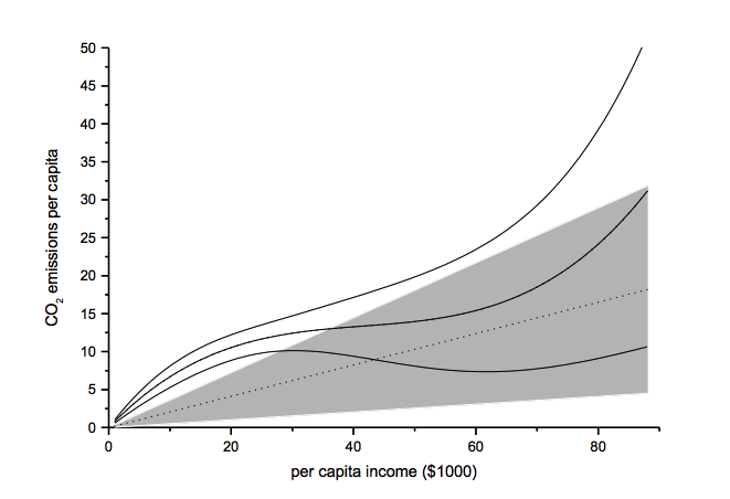
The functional form test examines the baseline model’s functional form assumption against a higher-order polynomial model. The two models should be nested to allow identical functional forms. As an example, we analyze the ‘environmental Kuznets curve’ prediction, which suggests the existence of an inverse u-shaped relation between per capita income and emissions.

Emissions and percapitaincome

Note: grey-shaded area represents confidence interval of baseline model

Another example of functional form testing is given in this review of Yield Curve Models:

http://jonathankinlay.com/2018/08/modeling-the-yield-curve/

Random Permutation Tests

Random permutation tests change specification assumptions repeatedly. Usually, researchers specify a model space and randomly and repeatedly select model from this model space. Examples:

  • sensitivity tests (Leamer 1978)
  • artificial measurement error (Plümper and Neumayer 2009)
  • sample split – attribute aggregation (Traunmüller and Plümper 2017)
  • multiple imputation (King et al. 2001)

We use Monte Carlo simulation to test the sensitivity of the performance of our Quantitative Equity strategy to changes in the price generation process and also in model parameters:

http://jonathankinlay.com/2017/04/new-longshort-equity/

Structured Permutation Tests

Structured permutation tests change a model assumption within a model space in a systematic way. Changes in the assumption are based on a rule, rather than random.  Possibilities here include:

  • sensitivity tests (Levine and Renelt)
  • jackknife test
  • partial demeaning test

Example: Jackknife Robustness Test

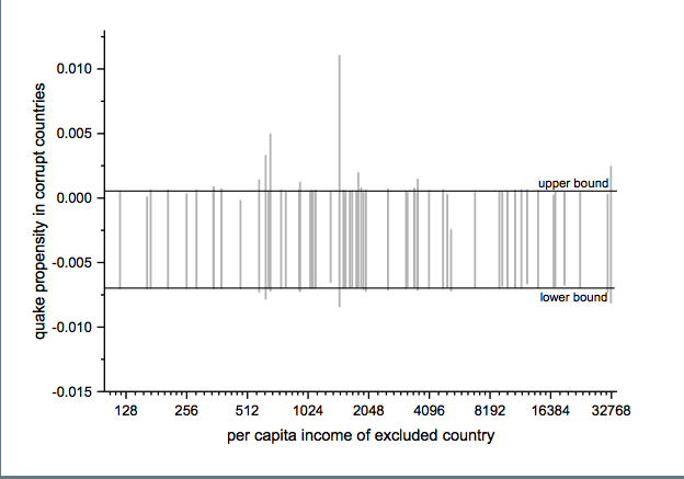
The jackknife robustness test is a structured permutation test that systematically excludes one or more observations from the estimation at a time until all observations have been excluded once. With a ‘group-wise jackknife’ robustness test, researchers systematically drop a set of cases that group together by satisfying a certain criterion – for example, countries within a certain per capita income range or all countries on a certain continent. In the example, we analyse the effect of earthquake propensity on quake mortality for countries with democratic governments, excluding one country at a time. We display the results using per capita income as information on the x-axes.

jackknife

Upper and lower bound mark the confidence interval of the baseline model.

Robustness Limit Tests

Robustness limit tests provide a way of analyzing structured permutation tests. These tests ask how much a model specification has to change to render the effect of interest non-robust. Some examples of robustness limit testing approaches:

  • unobserved omitted variables (Rosenbaum 1991)
  • measurement error
  • under- and overrepresentation
  • omitted variable correlation

For an example of limit testing, see this post on a review of the Lognormal Mixture Model:

http://jonathankinlay.com/2018/08/the-lognormal-mixture-variance-model/

Summary on Robustness Testing

Robustness tests have become an integral part of research methodology. Robustness tests allow to study the influence of arbitrary specification assumptions on estimates. They can identify uncertainties that otherwise slip the attention of empirical researchers. Robustness tests offer the currently most promising answer to model uncertainty.

Building Systematic Strategies – A New Approach

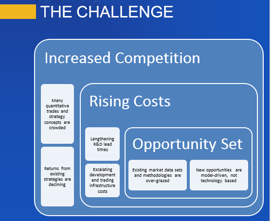
Anyone active in the quantitative space will tell you that it has become a great deal more competitive in recent years.  Many quantitative trades and strategies are a lot more crowded than they used to be and returns from existing  strategies are on the decline.

THE CHALLENGE

The Challenge

Meanwhile, costs have been steadily rising, as the technology arms race has accelerated, with more money being spent on hardware, communications and software than ever before.  As lead times to develop new strategies have risen, the cost of acquiring and maintaining expensive development resources have spiraled upwards.  It is getting harder to find new, profitable strategies, due in part to the over-grazing of existing methodologies and data sets (like the E-Mini futures, for example). There has, too, been a change in the direction of quantitative research in recent years.  Where once it was simply a matter of acquiring the fastest pipe to as many relevant locations as possible, the marginal benefit of each extra $ spent on infrastructure has since fallen rapidly.  New strategy research and development is now more model-driven than technology driven.


THE OPPORTUNITY

The Opportunity

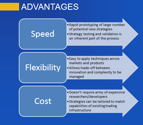
What is needed at this point is a new approach:  one that accelerates the process of identifying new alpha signals, prototyping and testing new strategies and bringing them into production, leveraging existing battle-tested technologies and trading platforms.


GENETIC PROGRAMMING

Genetic programming, which has been around since the 1990’s when its use was pioneered in proteomics, enjoys significant advantages over traditional research and development methodologies.

GP

GP is an evolutionary-based algorithmic methodology in which a system is given a set of simple rules, some data, and a fitness function that produces desired outcomes from combining the rules and applying them to the data.   The idea is that, by testing large numbers of possible combinations of rules, typically in the  millions, and allowing the most successful rules to propagate, eventually we will arrive at a strategy solution that offers the required characteristics.

ADVANTAGES OF GENETIC PROGRAMMING

AdvantagesThe potential benefits of the GP approach are considerable:  not only are strategies developed much more quickly and cost effectively (the price of some software and a single CPU vs. a small army of developers), the process is much more flexible. The inflexibility of the traditional approach to R&D is one of its principle shortcomings.  The researcher produces a piece of research that is subsequently passed on to the development team.  Developers are usually extremely rigid in their approach: when asked to deliver X, they will deliver X, not some variation on X.  Unfortunately research is not an exact science: what looks good in a back-test environment may not pass muster when implemented in live trading.  So researchers need to “iterate around” the idea, trying different combinations of entry and exit logic, for example, until they find a variant that works.  Developers are lousy at this;  GP systems excel at it.

CHALLENGES FOR THE GENETIC PROGRAMMING APPROACH

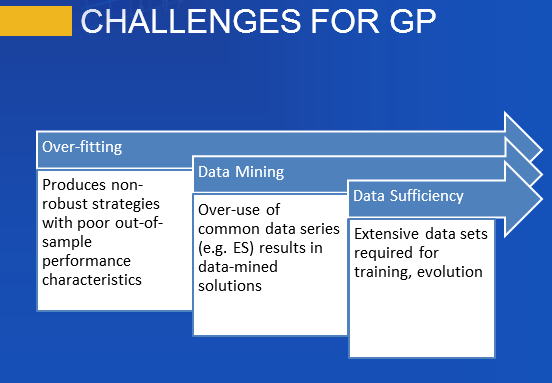
So enticing are the potential benefits of GP that it begs the question as to why the approach hasn’t been adopted more widely.  One reason is the strong preference amongst researchers for an understandable – and testable – investment thesis.  Researchers – and, more importantly, investors –  are much more comfortable if they can articulate the premise behind a strategy.  Even if a trade turns out to be a loser, we are generally more comfortable buying a stock on the supposition of, say,  a positive outcome of a pending drug trial, than we are if required to trust the judgment of a black box, whose criteria are inherently unobservable.

GP Challenges

Added to this, the GP approach suffers from three key drawbacks:  data sufficiency, data mining and over-fitting.  These are so well known that they hardly require further rehearsal.  There have been many adverse outcomes resulting from poorly designed mechanical systems curve fitted to the data. Anyone who was active in the space in the 1990s will recall the hype over neural networks and the over-exaggerated claims made for their efficacy in trading system design.  Genetic Programming, a far more general and powerful concept,  suffered unfairly from the ensuing adverse publicity, although it does face many of the same challenges.

A NEW APPROACH

I began working in the field of genetic programming in the 1990’s, with my former colleague Haftan Eckholdt, at that time head of neuroscience at Yeshiva University, and we founded a hedge fund, Proteom Capital, based on that approach (large due to Haftan’s research).  I and my colleagues at Systematic Strategies have continued to work on GP related ideas over the last twenty years, and during that period we have developed a methodology that address the weaknesses that have held back genetic programming from widespread adoption.

Advances

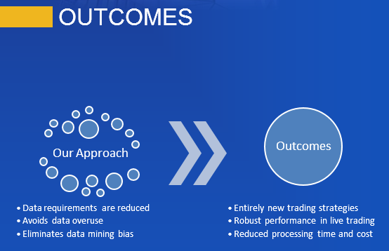
Firstly, we have evolved methods for transforming original data series that enables us to avoid over-using the same old data-sets and, more importantly, allows new patterns to be revealed in the underlying market structure.   This effectively eliminates the data mining bias that has plagued the GP approach. At the same time, because our process produces a stronger signal relative to the background noise, we consume far less data – typically no more than a couple of years worth.

Secondly, we have found we can enhance the robustness of prototype strategies by using double-blind testing: i.e. data sets on which the performance of the model remains unknown to the machine, or the researcher, prior to the final model selection.

Finally, we are able to test not only the alpha signal, but also multiple variations of the trade expression, including different types of entry and exit logic, as well as profit targets and stop loss constraints.

OUTCOMES:  ROBUST, PROFITABLE STRATEGIES

outcomes

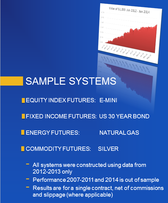
Taken together, these measures enable our GP system to produce strategies that not only have very high performance characteristics, but are also extremely robust.  So, for example, having constructed a model using data only from the continuing bull market in equities in 2012 and 2013, the system is nonetheless capable of producing strategies that perform extremely well when tested out of sample over the highly volatility bear market conditions of 2008/09.

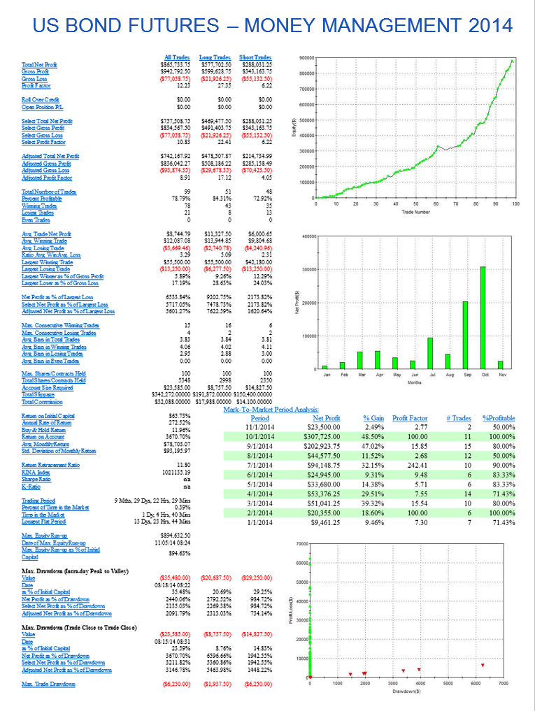
So stable are the results produced by many of the strategies, and so well risk-controlled, that it is possible to deploy leveraged money-managed techniques, such as Vince’s fixed fractional approach.  Money management schemes take advantage of the high level of consistency in performance to increase the capital allocation to the strategy in a way that boosts returns without incurring a high risk of catastrophic loss.  You can judge the benefits of applying these kinds of techniques in some of the strategies we have developed in equity, fixed income, commodity and energy futures which are described below.

CONCLUSION

After 20-30 years of incubation, the Genetic Programming approach to strategy research and development has come of age. It is now entirely feasible to develop trading systems that far outperform the overwhelming majority of strategies produced by human researchers, in a fraction of the time and for a fraction of the cost.

SAMPLE GP SYSTEMS

Sample

SSALGOTRADING AD

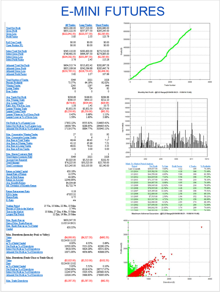
emini    emini MM

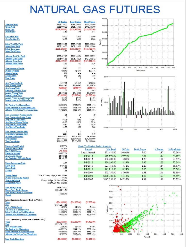
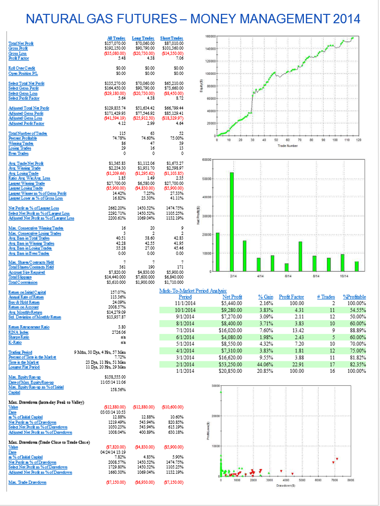
NG  NG MM

SI MMSI

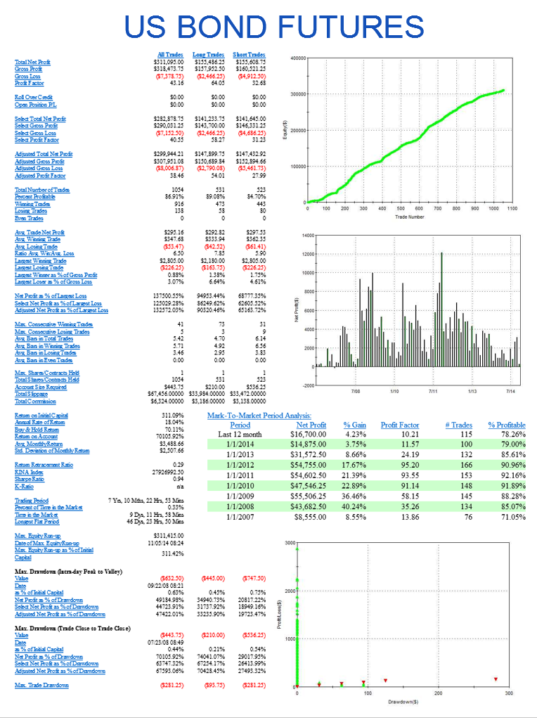
US US MM


Creating Robust, High-Performance Stock Portfolios

Summary

In this article, I am going to look at how stock portfolios should be constructed that best meet investment objectives.

The theoretical and practical difficulties of the widely adopted Modern Portfolio Theory approach limits its usefulness as a tool for portfolio construction.

MPT portfolios typically produce disappointing out-of-sample results, and will often underperform a naïve, equally-weighted stock portfolio.

The article introduces the concept of robust portfolio construction, which leads to portfolios that have more stable performance characteristics, including during periods of high volatility or market corrections.

The benefits of this approach include risk-adjusted returns that substantially exceed those of traditional portfolios, together with much lower drawdowns and correlations.

Market Timing

In an earlier article, I discussed how investors can enhance returns through the strategic use of market timing techniques to step out of the market during difficult conditions.

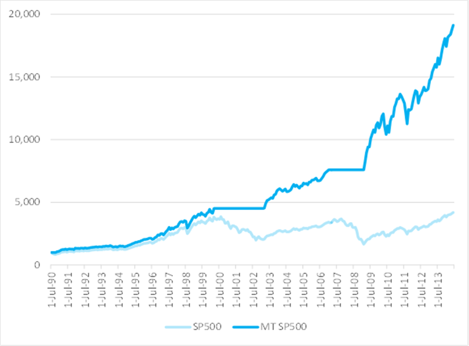
To emphasize the impact of market timing on investment returns, I have summarized in the chart below how a $1,000 investment would have grown over the 25-year period from July 1990 to June 2014. In the baseline scenario, we assume that the investment is made in a fund that tracks the S&P 500 Index and held for the full term. In the second scenario, we look at the outcome if the investor had stepped out of the market during the market downturns from March 2000 to Feb 2003 and from Jan 2007 to Feb 2009.

Fig. 1: Value of $1,000 Jul 1990-Jun 2014 – S&P 500 Index with and without Market Timing

Source: Yahoo Finance, 2014

After 25 years, the investment under the second scenario would have been worth approximately 5x as much as in the baseline scenario. Of course, perfect market timing is unlikely to be achievable. The best an investor can do is employ some kind of market timing indicator, such as the CBOE VIX index, as described in the previous article.

Equity Long Short

For those who mistrust the concept of market timing or who wish to remain invested in the market over the long term regardless of short-term market conditions, an alternative exists that bears consideration.

The equity long/short strategy, in which the investor buys certain stocks while shorting others, is a concept that reputedly originated with Alfred Jones in the 1940s. A long/short equity portfolio seeks to reduce overall market exposure, while profiting from stock gains in the long positions and price declines in the short positions. The idea is that the investor’s equity investments in the long positions are hedged to some degree against a general market decline by the offsetting short positions, from which the concept of a hedge fund is derived.

SSALGOTRADING AD

There are many variations on the long/short theme. Where the long and short positions are individually matched, the strategy is referred to as pairs trading. When the portfolio composition is structured in a way that the overall market exposure on the short side equates to that of the long side, leaving zero net market exposure, the strategy is typically referred to as market-neutral. Variations include dollar-neutral, where the dollar value of aggregate long and short positions is equalized, and beta-neutral, where the portfolio is structured in a way to yield a net zero overall market beta. But in the great majority of cases, such as, for example, in 130/30 strategies, there is a residual net long exposure to the market. Consequently, for the most part, long/short strategies are correlated with the overall market, but they will tend to outperform long-only strategies during market declines, while underperforming during strong market rallies.

Modern Portfolio Theory

Theories abound as to the best way to construct equity portfolios. The most commonly used approach is mean-variance optimization, a concept developed in the 1950s by Harry Markovitz (other more modern approaches include, for example, factor models or CVAR – conditional value at risk).

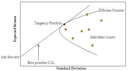
If we plot the risk and expected return of the assets under consideration, in what is referred to as the investment opportunity set, we see a characteristic “bullet” shape, the upper edge of which is called the efficient frontier (See Fig. 2). Assets on the efficient frontier produce the highest level of expected return for a given level of risk. Equivalently, a portfolio lying on the efficient frontier represents the combination offering the best possible expected return for a given risk level. It transpires that for efficient portfolios, the weights to be assigned to individual assets depend only on the volatilities of the individual assets and the correlation between them, and can be determined by simple linear programming. The inclusion of a riskless asset (such as US T-bills) allows us to construct the Capital Market Line, shown in the figure, which is tangent to the efficient frontier at the portfolio with the highest Sharpe Ratio, which is consequently referred to as the Tangency or Optimal Portfolio.

Fig. 2: Investment Opportunity Set and Efficient Frontier

Source: Wikipedia

Paradise Lost

Elegant as it is, MPT is open to challenge as a suitable basis for constructing investment portfolios. The Sharpe Ratio is often an inadequate representation of the investor’s utility function – for example, a strategy may have a high Sharpe Ratio but suffer from large drawdowns, behavior unlikely to be appealing to many investors. Of greater concern is the assumption of constant correlation between the assets in the investment universe. In fact, expected returns, volatilities and correlations fluctuate all the time, inducing changes in the shape of the efficient frontier and the composition of the optimal portfolio, which may be substantial. Not only is the composition of the optimal portfolio unstable, during times of financial crisis, all assets tend to become positively correlated and move down together. The supposed diversification benefit of MPT breaks down when it is needed the most.

I want to spend a little time on these critical issues before introducing a new methodology for portfolio construction. I will illustrate the procedure using a limited investment universe consisting of the dozen stocks listed below. This is, of course, a much more restricted universe than would typically apply in practice, but it does provide a span of different sectors and industries sufficient for our purpose.

Adobe Systems Inc. (NASDAQ:ADBE)
E. I. du Pont de Nemours and Company (NYSE:DD)
The Dow Chemical Company (NYSE:DOW)
Emerson Electric Co. (NYSE:EMR)
Honeywell International Inc. (NYSE:HON)
International Business Machines Corporation (NYSE:IBM)
McDonald’s Corp. (NYSE:MCD)
Oracle Corporation (NYSE:ORCL)
The Procter & Gamble Company (NYSE:PG)
Texas Instruments Inc. (NASDAQ:TXN)
Wells Fargo & Company (NYSE:WFC)
Williams Companies, Inc. (NYSE:WMB)

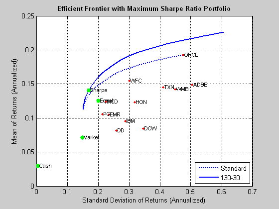
If we follow the procedure outlined in the preceding section, we arrive at the following depiction of the investment opportunity set and efficient frontier. Note that in the following, the S&P 500 index is used as a proxy for the market portfolio, while the equal portfolio designates a portfolio comprising identical dollar amounts invested in each stock.

Fig. 3: Investment Opportunity Set and Efficient Frontiers for the 12-Stock Portfolio

Source: MathWorks Inc.

As you can see, we have derived not one, but two, efficient frontiers. The first is the frontier for standard portfolios that are constrained to be long-only and without use of leverage. The second represents the frontier for 130/30 long-short portfolios, in which we permit leverage of 30%, so that long positions are overweight by a total of 30%, offset by a 30% short allocation. It turns out that in either case, the optimal portfolio yields an average annual return of around 13%, with annual volatility of around 17%, producing a Sharpe ratio of 0.75.

So far so good, but here, of course, we are estimating the optimal portfolio using the entire data set. In practice, we will need to estimate the optimal portfolio with available historical data and rebalance on a regular basis over time. Let’s assume that, starting in July 1995 and rolling forward month by month, we use the latest 60 months of available data to construct the efficient frontier and optimal portfolio.

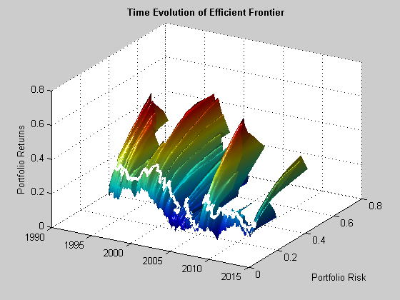
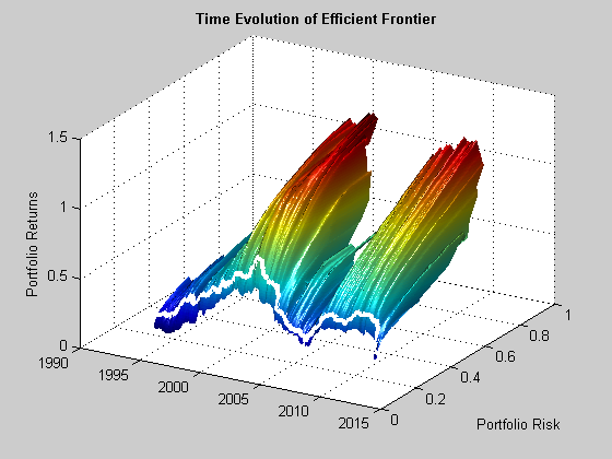
Fig. 4 below illustrates the enormous variation in the shape of the efficient frontier over time, and in the risk/return profile of the optimal long-only portfolio, shown as the white line traversing the frontier surface.

Fig. 4: Time Evolution of the Efficient Frontier and Optimal Portfolio

Source: MathWorks Inc.

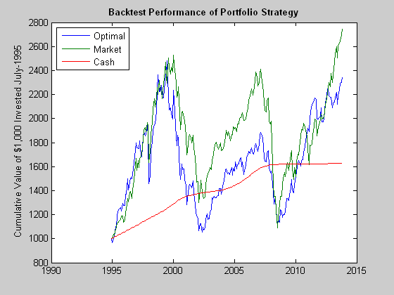
We see in Fig. 5 that the outcome of using the MPT approach is hardly very encouraging: the optimal long-only portfolio underperforms the market both in aggregate, over the entire back-test period, and consistently during the period from 2000-2011. The results for a 130/30 portfolio (not shown) are hardly an improvement, as the use of leverage, if anything, has a tendency to exacerbate portfolio turnover and other undesirable performance characteristics.

Fig. 5: Value of $1,000: Optimal Portfolio vs. S&P 500 Index, Jul 1995-Jun 2014

Source: MathWorks Inc.

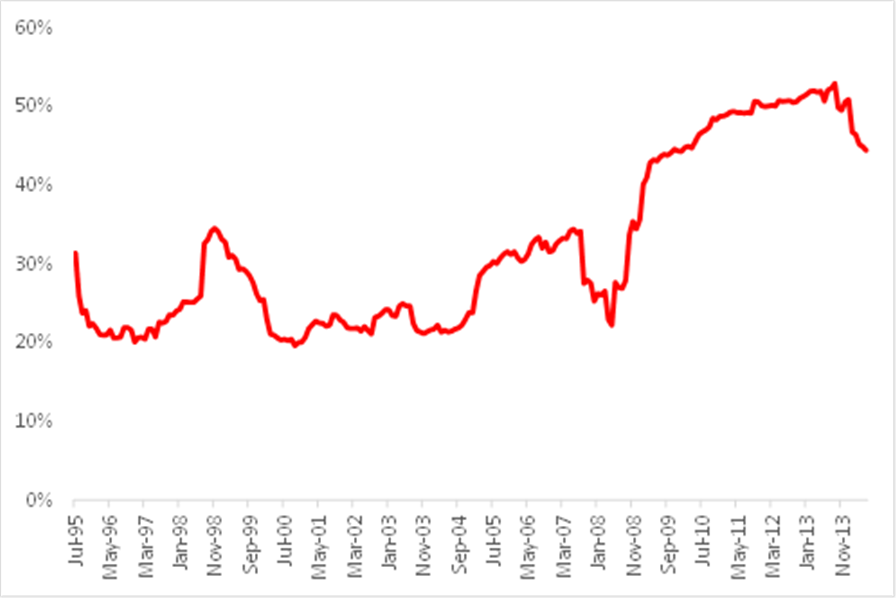
Part of the reason for the poor performance of the optimal portfolio lies with the assumption of constant correlation. In fact, as illustrated in Fig 6, the average correlation between the monthly returns in the twelve stocks in our universe has fluctuated very substantially over the last twenty years, ranging from a low of just over 20% to a high in excess of 50%, with an annual volatility of 38%. Clearly, the assumption of constant correlation is unsafe.

Fig. 6: Average Correlation, Jul 1995-Jun 2014

Source: Yahoo Finance, 2014

To add to the difficulties, researchers have found that the out of sample performance of the naïve portfolio, in which equal dollar value is invested in each stock, is typically no worse than that of portfolios constructed using techniques such as mean-variance optimization or factor models1. Due to the difficulty of accurately estimating asset correlations, it would require an estimation window of 3,000 months of historical data for a portfolio of only 25 assets to produce a mean-variance strategy that would outperform an equally-weighted portfolio!

Without piling on the agony with additional concerns about the MPT methodology, such as the assumption of Normality in asset returns, it is already clear that there are significant shortcomings to the approach.

Robust Portfolios

Many attempts have been made by its supporters to address the practical limitations of MPT, while other researchers have focused attention on alternative methodologies. In practice, however, it remains a challenge for any of the common techniques in use today to produce portfolios that will consistently outperform a naïve, equally-weighted portfolio. The approach discussed here represents a radical departure from standard methods, both in its objectives and in its methodology. I will discuss the general procedure without getting into all of the details, some of which are proprietary.

Let us revert for a moment to the initial discussion of market timing at the start of this article. We showed that if only we could time the market and step aside during major market declines, the outcome for the market portfolio would be a five-fold improvement in performance over the period from Aug 1990 to Jun 2014. In one sense, it would not take “much” to produce a substantial uplift in performance: what is needed is simply the ability to avoid the most extreme market drawdowns. We can identify this as a feature of what might be described as a “robust” portfolio, i.e. one with a limited tendency to participate in major market corrections. Focusing now on the general concept of “robustness”, what other characteristics might we want our ideal portfolio to have? We might consider, for example, some or all of the following:

  1. Ratio of total returns to max drawdown
  2. Percentage of profitable days
  3. Number of drawdowns and average length of drawdowns
  4. Sortino ratio
  5. Correlation to perfect equity curve
  6. Profit factor (ratio of gross profit to gross loss)
  7. Variability in average correlation

The list is by no means exhaustive or prescriptive. But these factors relate to a common theme, which we may characterize as robustness. A portfolio or strategy constructed with these criteria in mind is likely to have a very different composition and set of performance characteristics when compared to an optimal portfolio in the mean-variance sense. Furthermore, it is by no means the case that the robustness of such a portfolio must come at the expense of lower expected returns. As we have seen, a portfolio which only produces a zero return during major market declines has far higher overall returns than one that is correlated with the market. If the portfolio can be constructed in a way that will tend to produce positive returns during market downturns, so much the better. In other words, what we are describing is a long/short portfolio whose correlation to the market adapts to market conditions, having a tendency to become negative when markets are in decline and positive when they are rising.

The first insight of this approach, then, is that we use different criteria, often multi-dimensional, to define optimality. These criteria have a tendency to produce portfolios that behave robustly, performing well during market declines or periods of high volatility, as well as during market rallies.

The second insight from the robust portfolio approach arises from the observation that, ideally, we would want to see much greater consistency in the correlations between assets in the investment universe than is typically the case for stock portfolios. Now, stock correlations are what they are and fluctuate as they will – there is not much one can do about that, at least directly. One solution might be to include other assets, such as commodities, into the mix, in an attempt to reduce and stabilize average asset correlations. But not only is this often undesirable, it is unnecessary – one can, in fact, reduce average correlation levels, while remaining entirely with the equity universe.

The solution to this apparent paradox is simple, albeit entirely at odds with the MPT approach. Instead of creating our portfolio on the basis of combining a group of stocks in some weighting scheme, we are first going to develop investment strategies for each of the stocks individually, before combining them into a portfolio. The strategies for each stock are designed according to several of the criteria of robustness we identified earlier. When combined together, these individual strategies will merge to become a portfolio, with allocations to each stock, just as in any other weighting scheme. And as with any other portfolio, we can set limits on allocations, turnover, or leverage. In this case, however, the resulting portfolio will, like its constituent strategies, display many of the desired characteristics of robustness.

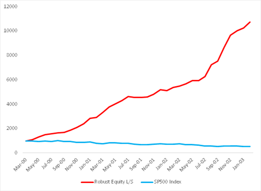
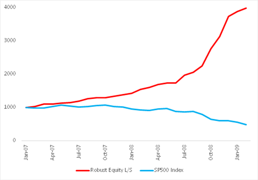
Let’s take a look at how this works out for our sample universe of twelve stocks. I will begin by focusing on the results from the two critical periods from March 2000 to Feb 2003 and from Jan 2007 to Feb 2009.

Fig. 7: Robust Equity Long/Short vs. S&P 500 index, Mar 2000-Feb 2003

Source: Yahoo Finance, 2014

Fig. 8: Robust Equity Long/Short vs. S&P 500 index, Jan 2007-Feb 2009

Source: Yahoo Finance, 2014

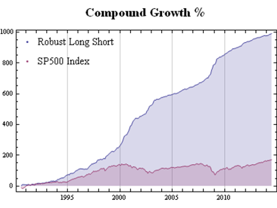
As might be imagined, given its performance during these critical periods, the overall performance of the robust portfolio dominates the market portfolio over the entire period from 1990:

Fig. 9: Robust Equity Long/Short vs. S&P 500 index, Aug 1990-Jun 2014

Source: Yahoo Finance, 2014

It is worth pointing out that even during benign market conditions, such as those prevailing from, say, the end of 2012, the robust portfolio outperforms the market portfolio on a risk-adjusted basis: while the returns are comparable for both, around 36% in total, the annual volatility of the robust portfolio is only 4.8%, compared to 8.4% for the S&P 500 index.

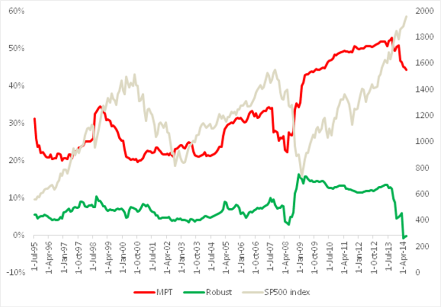
A significant benefit to the robust portfolio derives from the much lower and more stable average correlation between its constituent strategies, compared to the average correlation between the individual equities, which we considered before. As can be seen from Fig. 10, average correlation levels remained under 10% for the robust portfolio, compared to around 25% for the mean-variance optimal portfolio until 2008, rising only to a maximum value of around 15% in 2009. Thereafter, average correlation levels have drifted consistently in the downward direction, and are now very close to zero. Overall, average correlations are much more stable for the constituents in the robust portfolio than for those in the traditional portfolio: annual volatility at 12.2% is less than one-third of the annual volatility of the latter, 38.1%.

Fig. 10: Average Correlations Robust Equity Long/Short vs. S&P 500 index, Aug 1990-Jun 2014

Source: Yahoo Finance, 2014

The much lower average correlation levels mean that it is possible to construct fully diversified portfolios in the robust portfolio framework with fewer assets than in the traditional MPT framework. Put another way, a robust portfolio with a small number of assets will typically produce higher returns with lower volatility than a traditional, optimal portfolio (in the MPT sense) constructed using the same underlying assets.

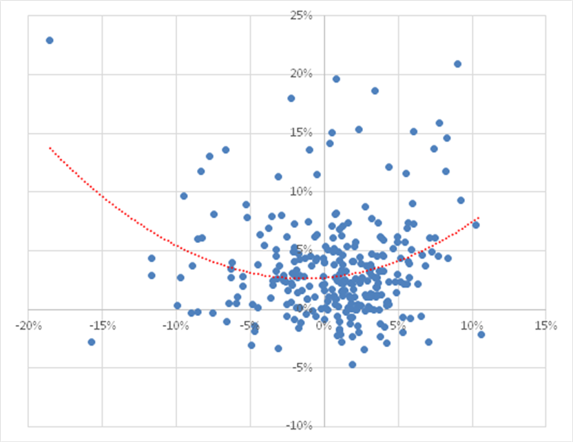
In terms of correlation of the portfolio itself, we find that over the period from Aug 1990 to June 2014, the robust portfolio exhibits close to zero net correlation with the market. However, the summary result disguises yet another important advantage of the robust portfolio. From the scatterplot shown in Fig. 11, we can see that, in fact, the robust portfolio has a tendency to adjust its correlation according to market conditions. When the market is moving positively, the robust portfolio tends to have a positive correlation, while during periods when the market is in decline, the robust portfolio tends to have a negative correlation.

Fig. 11: Correlation between Robust Equity Long/Short vs. S&P 500 index, Aug 1990-Jun 2014

Source: Yahoo Finance, 2014

Optimal Robust Portfolios

The robust portfolio referenced in our discussion hitherto is a naïve portfolio with equal dollar allocations to each individual equity strategy. What happens if we apply MPT to the equity strategy constituents and construct an “optimal” (in the mean-variance sense) robust portfolio?

The results from this procedure are summarized in Fig. 12, which shows the evolution of the efficient frontier, traversed by the risk/return path of the optimal robust portfolio. Both show considerable variability. In fact, however, both the frontier and optimal portfolio are far more stable than their equivalents for the traditional MPT strategy.

Fig. 12: Time Evolution of the Efficient Frontier and Optimal Robust Portfolio

Source: MathWorks Inc.

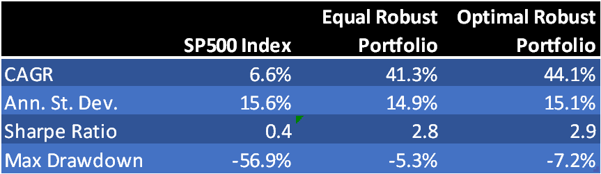
Fig. 13 compares the performance of the naïve robust portfolio and optimal robust portfolio. The optimal portfolio does demonstrate a small, material improvement in risk-adjusted returns, but at the cost of an increase in the maximum drawdown. It is an open question as to whether the modest improvement in performance is sufficient to justify the additional portfolio turnover and commensurate trading cost and operational risk. The incremental benefits are relatively minor, because the equally weighted portfolio is already well-diversified due to the low average correlation in its constituent strategies.

Fig. 13: Naïve vs. Optimal Robust Portfolio Performance Aug 1990-Jun 2014

Source: Yahoo Finance, 2014

Conclusion

The limitations of MPT in terms of its underlying assumptions and implementation challenges limits its usefulness as a practical tool for investors looking to construct equity portfolios that will enable them to achieve their investment objectives. Rather than seeking to optimize risk-adjusted returns in the traditional way, investors may be better served by identifying important characteristics of strategy robustness and using these to create strategies for individual equities that perform robustly across a wide range of market conditions. By constructing portfolios composed of such strategies, rather than using the underlying equities, investors may achieve higher, more stable returns under a broad range of market conditions, including periods of high volatility or market drawdown.

1 Optimal Versus Naive Diversification: How Inefficient is the 1/N Portfolio Strategy?, Victor DeMiguel, Lorenzo Garlappi and Raman Uppal, The Review of Financial Studies, Vol. 22, Issue 5, 2007.

More on Strategy Robustness

Commentators have made the point that a high % win rate is not enough.

Yes, you obviously want to pay attention to other performance metrics also, such as profit factor. In fact, there is no reason why you shouldn’t consider an objective function that explicitly combines various desirable performance measures, for example:

net profit * % win rate * profit factor

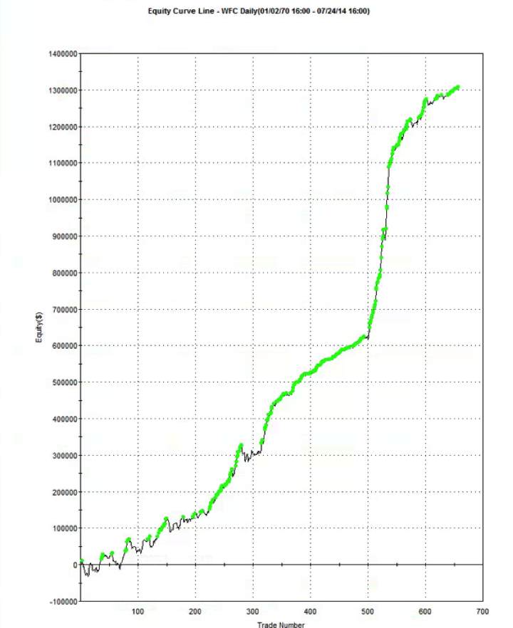
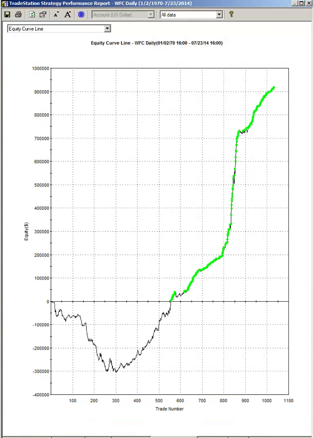
Another approach is to build the model using a data set spanning a different period. I did this with WFC using data from 1990, rather than 1970. Not only was the performance from 1990-2014 better, so too was the performance during the OOS period 1970-1989.  Profit factor was 2.49 and %Win rate was 70% across the 44 year period from 1970.  For the period from 1990, the performance metrics increase to 3.04 and 73%, respectively.

SSALGOTRADING AD

So in this case, it appears, a most robust strategy resulted from using less data, rather than more.  At first this appears counterintuitive. But it’s quite possible for a strategy to be over-condition on behavior that is no longer relevant to the market today. Eliminating such conditioning can sometimes enable strategies to emerge that have greater longevity.

WFC from 1970-2014 (1990 data)

Performance

Optimizing Strategy Robustness

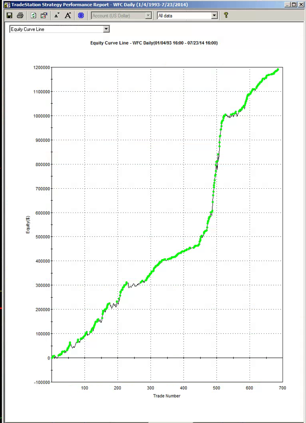
Below is the equity curve for an equity strategy I developed recently, implemented in WFC.  The results appear outstanding:  no losing years in over 20 years, profit factor of 2.76 and average win rate of 75%.  Out-of-sample results (double blind) for 2013 and 2014:  net returns of 27% and 16% YTD.

WFC from 1993-2014


So far so good. However, if we take a step back through the earlier out of sample period, from 1970, the picture is rather less rosy:


WFC from 1970-2014


Now, at this point, some of you will be saying:  nothing to see here – it’s obviously just curve fitting.  To which I would respond that I have seen successful strategies, including several hedge fund products, with far shorter and less impressive back-tests than the initial 20-year history I showed above.

SSALGOTRADING AD

That said, would you be willing to take the risk of trading a strategy such as this one?  I would not:  at the back of my mind would always be the concern that the market might easily revert to the conditions that applied during the 1970s and 1980’s.  I expect many investors would share that concern.

But to the point of this post:  most strategies are designed around the criterion of maximizing net profit.  Occasionally you might come across someone who has considered risk, perhaps in the form of drawdown, or Sharpe ratio.  But, in general, it’s all about optimizing performance.

Suppose that, instead of maximizing performance, your objective was to maximize the robustness of the strategy.  What criteria would you use?

In my own research, I have used a great many different objective functions, often multi-dimensional.  Correlation to the perfect equity curve, net profit / max drawdown and Sortino ratio are just a few examples.  But if I had to guess, I would say that the criteria that tends to produce the most robust strategies and reliable out of sample performance is the maximization of the win rate, subject to a minimum number of trades.

I am not aware of a great deal of theory on this topic. I would be interested to learn of other readers’ experience.


How Not to Develop Trading Strategies – A Cautionary Tale

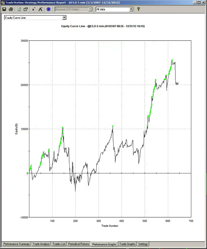
In his post on Multi-Market Techniques for Robust Trading Strategies (http://www.adaptrade.com/Newsletter/NL-MultiMarket.htm) Michael Bryant of Adaptrade discusses some interesting approaches to improving model robustness. One is to use data from several correlated assets to build the model, on the basis that if the algorithm works for several assets with differing price levels, that would tend to corroborate the system’s robustness. The second approach he advocates is to use data from the same asset series at different bars lengths. The example he uses @ES.D at 5, 7 and 9 minute bars. The argument in favor of this approach is the same as for the first, albeit in this case the underlying asset is the same.

I like Michael’s idea in principle, but I wanted to give you a sense of what can all too easily go wrong with GP modeling, even using techniques such as multi-time frame fitting and Monte Carlo simulation to improve robustness testing.

In the chart below I have extended the analysis back in time, beyond the 2011-2012 period that Michael used to build his original model. As you can see, most of the returns are generated in-sample, in the 2011-2012 period. As we look back over the period from 2007-2010, the results are distinctly unimpressive – the strategy basically trades sideways for four years.

Adaptrade ES Strategy in Multiple Time Frames


How do Do It Right

In my view, there is only one, safe way to use GP to develop strategies. Firstly, you need to use a very long span of data – as much as possible, to fit your model. Only in this way can you ensure that the model has encountered enough variation in market conditions to stand a reasonable chance of being able to adapt to changing market conditions in future.

SSALGOTRADING AD

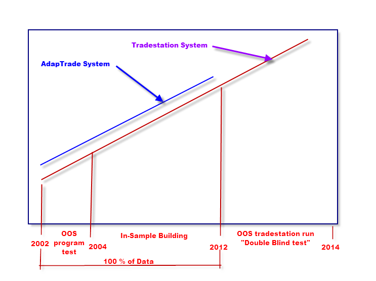
Secondly, you need to use two OOS period. The first OOS span of data, drawn from the start of the data series, is used in the normal way, to visually inspect the performance of the model. But the second span of OOS data, from more recent history, is NOT examined before the model is finalized. This is really important. Products like Adaptrade make it too easy for the system designer to “cheat”, by looking at the recent performance of his trading system “out of sample” and selecting models that do well in that period. But the very process of examining OOS performance introduces bias into the system. It would be like adding a line of code saying something like:

IF (model performance in OOS period > x) do the following….

I am quite sure if I posted a strategy with a line of code like that in it, it would immediately be shot down as being blatantly biased, and quite rightly so. But, if I look at the recent “OOS” performance and use it to select the model, I am effectively doing exactly the same thing.

That is why it is so important to have a second span of OOS data that it not only not used to build the model, but also is not used to assess performance, until after the final model selection is made. For that reason, the second OOS period is referred to as a “double blind” test.

That’s the procedure I followed to build my futures daytrading strategy: I used as much data as possible, dating from 2002. The first 20% of the each data set was used for normal OOS testing. But the second set of data, from Jan 2012 onwards, was my double-blind data set. Only when I saw that the system maintained performance in BOTH OOS periods was I reasonably confident of the system’s robustness.

DoubleBlind

This further explains why it is so challenging to develop higher frequency strategies using GP. Running even a very fast GP modeling system on a large span of high frequency data can take inordinate amounts of time.

The longest span of 5-min bar data that a GP system can handle would typically be around 5-7 years. This is probably not quite enough to build a truly robust system, although if you pick you time span carefully it might be (I generally like to use the 2006-2011 period, which has lots of market variation).

For 15 minute bar data, a well-designed GP system can usually handle all the available data you can throw at it – from 1999 in the case of the Emini, for instance.

Why I don’t Like Fitting Models over Short Time Spans

The risks of fitting models to data in short time spans are intuitively obvious. If you happen to pick a data set in which the market is in a strong uptrend, then your model is going to focus on that kind of market behavior. Subsequently, when the trend changes, the strategy will typically break down.
Monte Carlo simulation isn’t going to change much in this situation: sure, it will help a bit, perhaps, but since the resampled data is all drawn from the same original data set, in most cases the simulated paths will also show a strong uptrend – all that will be shown is that there is some doubt about the strength of the trend. But a completely different scenario, in which, say, the market drops by 10%, is unlikely to appear.

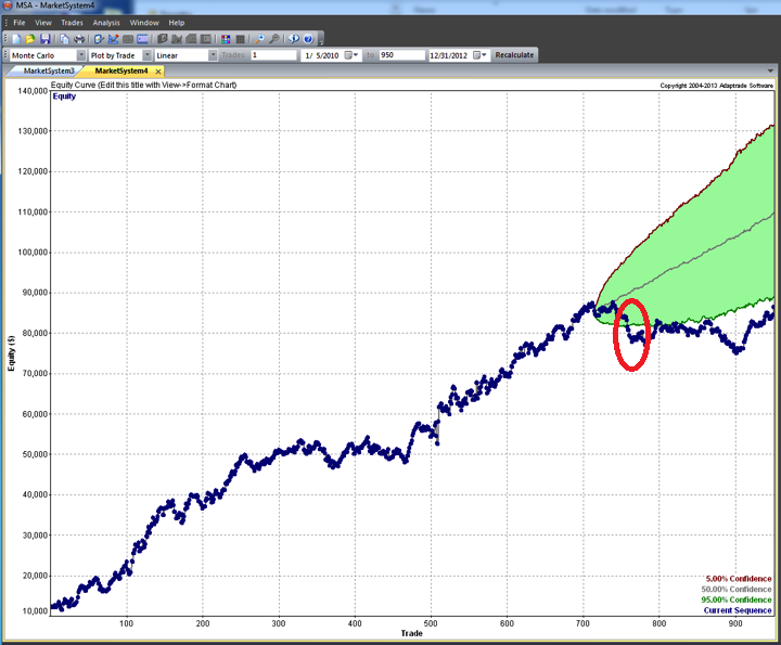
One possible answer to that problem, recommended by some system developers, is simply to rebuild the model when a breakdown is detected. While it’s true that a product like MSA can make detection easier, rebuilding the model is another question altogether. There is no guarantee that the kind of model that has worked hitherto can be re-tooled to work once again. In fact, there may be no viable trading system that can handle the new market dynamics.

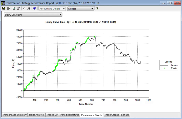
Here is a case in point. We have a system that works well on 10 min bars in TF.D up until around May 2012, when MSA indicates a breakdown in strategy performance.

TF.F Monte Carlo

So now we try to fit a new model, along the pattern of the original model, taking account some of the new data.  But it turns out to be just a Band-Aid – after a few more data points the strategy breaks down again, irretrievably.

TF EC 1

This is typical of what often happens when you use GP to build a model using s short span of data. That’s why I prefer to use a long time span, even at lower frequency. The chances of being able to build a robust system that will adapt well to changing market conditions are much higher.

A Robust Emini Trading System

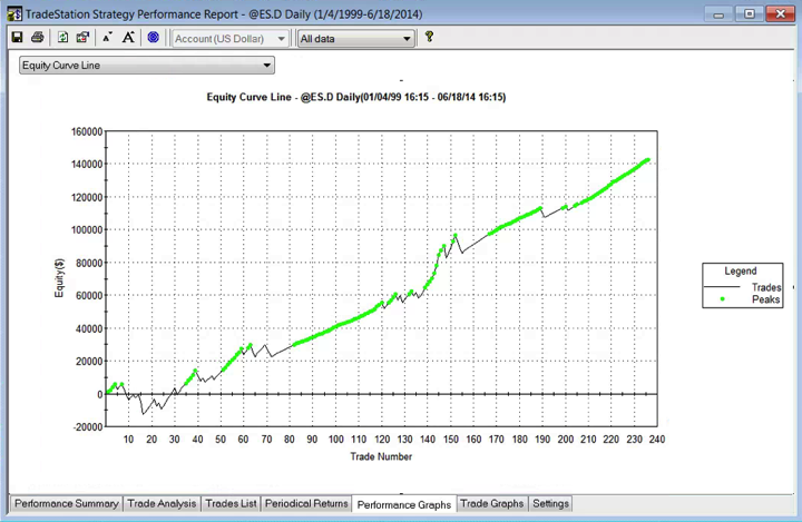
Here, for example is a GP system build on daily data in @ES.D from 1999 to 2011 (i.e. 2012 to 2014 is OOS).

ES.D EC