Deep Learning for Volatility Surface Repair

A self-contained synthetic benchmark of a small mask-conditional CNN against calendar-projected linear interpolation and a per-slice SVI fit.

A volatility surface marker is rarely a clean rectangle of quotes. Strikes go unobserved during illiquid hours, wings get crossed and then erased, broker stripes drop out across an entire maturity, and weeklies arrive at the desk with random missingness on top of base quote noise. Anyone calibrating an SVI surface or running an SSVI fit operationally is doing it on top of an upstream repair step, whether that step is explicit or not. The repair step is usually some flavour of local interpolation, sometimes followed by a no-arbitrage projection, sometimes pre-empted by a model-based smoother.

The question I want to put a number on is whether a small learned model can compete with the local approach in this repair role. The reason to ask is that a learned model, in principle, knows something about the joint structure of plausible volatility surfaces that a local interpolator does not — vol surfaces are not arbitrary functions on a (k, T) grid, they have term-structure shape, characteristic skew patterns, ATM smoothness — and a model that has seen a thousand surfaces should be able to use that prior to improve on local interpolation, especially where local data is thin.

The reason to be sceptical is that local methods are very strong at what they do. Linear interpolation in (T, k) is unbiased, has no parameters to overfit, costs nothing operationally, and is hard to beat on smooth surfaces with reasonable observation density. Per-slice SVI gets you smile shape correctly even when only a handful of strikes are observed, provided the slice has enough quotes to fit. Beating both of those baselines requires that the learned prior contributes something local methods cannot — and the most plausible places for that to happen are when local data is too sparse for SVI to fit and too irregular for interpolation to fill the gap cleanly.

This note runs that experiment on synthetic data. It is deliberately a small CNN rather than a U-Net or a VAE, partly because that is the smallest interesting architecture for this problem, and partly because if a small model cannot establish a foothold here, the question of whether to build something larger has a clearer answer than if it can.

The full code is in vol_surface_repair.py; it runs on CPU in roughly four minutes.

Setup

Grid. Maturities and log-moneyness on a 13 × 17 grid: T \in [0.08, 2.0] (years), k \in [-0.45, 0.45]. All surfaces are stored as total variance w(k, T) = \sigma^2(k, T)\, T; evaluation metrics are computed in implied-vol units (\sigma) for interpretability.

Training surfaces. 1600 SSVI surfaces drawn from a fairly tight parameter range:

theta0 = U(0.010, 0.032)        # ATM total variance at front
theta_slope = U(0.020, 0.070)   # linear term in maturity
theta_curve = U(-0.006, 0.010)  # quadratic term
rho = U(-0.72, -0.18)           # skew
eta = U(0.55, 1.55)             # SSVI eta
gamma = U(0.18, 0.62)           # SSVI gamma

Calendar monotonicity is enforced on the clean target via cumulative maximum along T so the model is never rewarded for learning calendar arbitrage from the simulator. A 200-surface validation set, drawn from the same parameter range with different seeds, is held out for best-checkpoint selection.

Test surfaces. Two test families, each with 200 surfaces per cell and seeds independent of training:

  • Shifted SSVI — same generator with widened parameter ranges and an occasional maturity-localised bump. The generator is in-distribution in form but stress-tests the boundaries.
  • SABR-style event — a separate generator deliberately not identical to SSVI, with square-root maturity decay in ATM vol, stochastic skew term-structure, asymmetric wings, and occasional event-maturity bumps and kinks. This is the out-of-distribution test: smile structure that the model has never seen.

Both families are then perturbed by realistic quote noise (~18 bps in vol space, with wing- and front-end inflation) and masked according to one of two missingness regimes:

  • Regular — about 50% observation density, modest wing deletions, occasional broker-style stripes.
  • Adversarial — about 18% observation density, large contiguous wing or maturity holes, with a thin ATM spine and a few scattered anchors restored so the problem remains solvable but is genuinely sparse.

The result is a 2 × 2 evaluation: {shifted SSVI, SABR-event} × {regular, adversarial}. The motivation is to disentangle two different ways the repair task can be hard: hard because the model has not seen this surface family before, and hard because the available data is too sparse for any local method to cope.

Baselines. Two of them.

  • Calendar-projected linear interpolation: triangulated linear interpolation in (T, k) on observed total variance, with a nearest-neighbour fallback for points outside the convex hull, followed by a cumulative-maximum projection along T to enforce calendar monotonicity. Unparameterised, fast, hard to beat on smooth surfaces.
  • Per-slice SVI fit: at each maturity, a coarse raw-SVI grid search over (\rho, m, \sigma) with the best (a, b) solved in closed form by least squares. Faster than nonlinear least squares, adequate as a baseline. Followed by the same calendar projection as interpolation. This is the published-textbook approach to surface repair when you have enough quotes per slice.

Both baselines are evaluated on the same noisy/masked inputs as the CNN.

Model

The repair network is a four-layer 32-channel convolutional network with two output heads — a softplus mean head and a clipped log-variance head:

class RepairCNN(nn.Module):
   def __init__(self, in_channels=4, width=32):
       super().__init__()
       self.backbone = nn.Sequential(
           nn.Conv2d(in_channels, width, 3, padding=1), nn.SiLU(),
           nn.Conv2d(width, width, 3, padding=1), nn.SiLU(),
           nn.Conv2d(width, width, 3, padding=1), nn.SiLU(),
           nn.Conv2d(width, width, 3, padding=1), nn.SiLU(),
      )
       self.mean_head = nn.Conv2d(width, 1, 1)
       self.logvar_head = nn.Conv2d(width, 1, 1)

   def forward(self, x):
       z = self.backbone(x)
       mean = F.softplus(self.mean_head(z)) + 1e-5  # w / W_SCALE
       log_var = torch.clamp(self.logvar_head(z), -8.0, 1.5)
       return mean, log_var

The four input channels are the masked observed total variance (normalised by W_SCALE = 0.08), the binary observation mask, and two normalised coordinate channels for maturity and log-moneyness. The mean head outputs normalised total variance; the log-variance head produces a heteroscedastic uncertainty estimate.

The output space is total variance rather than implied vol. Both choices are defensible — a controlled experiment with the same training pipeline run in vol space gives essentially identical missing-point RMSE — and total variance has the practical advantage that calendar-arbitrage and butterfly-arbitrage diagnostics are natural in this space.

The loss is a weighted reconstruction term in the normalised w-space, plus a heteroscedastic Gaussian NLL (turned on after a 10-epoch warmup), plus a calendar-arbitrage penalty (penalising negative differences along T in real-w space), plus a small smoothness regulariser:

def repair_loss(mean_norm, log_var, target_norm, mask, cfg, use_nll):
   weights = 1.0 + (cfg.missing_weight - 1.0) * (1.0 - mask)
   sq = (mean_norm - target_norm)**2
   mse = torch.mean(weights * sq)
   loss = mse
   if use_nll and cfg.nll_weight:
       inv_var = torch.exp(-log_var)
       nll = 0.5 * torch.mean(weights * (sq * inv_var + log_var))
       loss = loss + cfg.nll_weight * nll
   if cfg.calendar_weight:
       loss = loss + cfg.calendar_weight * calendar_penalty_w(mean_norm)
   if cfg.smoothness_weight:
       loss = loss + cfg.smoothness_weight * smoothness_penalty(mean_norm)
   return loss

The missing-cell weight is 5x the observed-cell weight, so the model is explicitly graded on its repair quality rather than its ability to denoise observed quotes. The calendar weight is set to 80, which is high enough to drive raw calendar-violation rates into single digits at evaluation time but not so high that it dominates the reconstruction loss during training. The smoothness term is small (0.05 weight) and exists mainly to discourage high-frequency artefacts at the wings.

Training runs for 60 epochs in a single process with AdamW (lr 1e-3, wd 1e-4) and a cosine annealing schedule. The first 10 epochs run pure MSE; the NLL term turns on afterwards to give the variance head an MSE-stabilised mean to train against. A 200-surface validation set is used for best-checkpoint selection by missing-point RMSE in vol units. Batch size 128, gradient clipping at norm 1.0.

I will say a word about training duration because the result is more sensitive to it than I would like. With only 8 training epochs, the model’s missing-point RMSE on shifted SSVI / regular missing is 0.049 in vol units; at 60 epochs it is 0.018. The convergence is slow and the validation curve is still improving slightly at epoch 60. Sixty epochs is therefore a deliberate choice rather than a generous one — at that point the validation curve has flattened enough that further training mostly trades off in-distribution refinement against out-of-distribution generalisation, with no clear winner.

The 2 × 2 result

Headline numbers: missing-point RMSE in implied-vol units, mean ± standard error across 200 test surfaces per cell. Bold marks the best estimator per row, with ties (within one SE) bolded together.

CaseObs %CNNInterpSVI
Shifted SSVI / regular50.5%0.0184 ± 0.00100.0131 ± 0.00080.0191 ± 0.0048
Shifted SSVI / adversarial18.1%0.0527 ± 0.00240.0506 ± 0.00260.0540 ± 0.0123
SABR-event / regular50.4%0.0671 ± 0.00130.0248 ± 0.00110.0189 ± 0.0021
SABR-event / adversarial17.7%0.0960 ± 0.00110.0679 ± 0.00190.0784 ± 0.0089

Four cells, four different stories.

Shifted SSVI / regular. Calendar-projected linear interpolation wins outright: 0.013 versus the CNN’s 0.018. The surfaces here are smooth, the parameter shifts from the training distribution are modest, and roughly half the grid is observed. There is little for a learned prior to add: the local data is dense enough that triangulated interpolation captures essentially all the recoverable structure. The CNN is 40% worse, well outside one SE.

Shifted SSVI / adversarial. The CNN and interpolation are statistically tied (0.053 vs 0.051, within one SE of each other). With observation density at 18% and large contiguous holes, neither method has a clean run, but the CNN’s learned prior on smile shape brings it back into the same neighbourhood as interpolation. The SVI fit is also competitive here, although noisier across surfaces because individual maturity slices sometimes have too few quotes to fit reliably.

SABR-event / regular. SVI wins narrowly (0.019 vs interpolation’s 0.025), the CNN comes in third at 0.067. This is the cell that distinguishes baselines: SVI fits the local smile structure correctly slice-by-slice and pays no penalty for the SABR family being out-of-distribution because it is a per-slice model with no cross-slice prior to mislead it. The CNN, trained only on SSVI surfaces, has learned a prior that does not transfer cleanly to the asymmetric-wings, event-kink SABR family. It is 2.5× worse than SVI here.

SABR-event / adversarial. Interpolation wins (0.068 vs the CNN’s 0.096), with SVI in the middle at 0.078 and noisy because slice-level data is too sparse to fit consistently. The dominant error source for the CNN here is generalisation, not data scarcity. Even with adversarial missingness — exactly the case where one might hope a learned prior contributes most — the OOD penalty dominates.

The pattern across cells is consistent. The CNN is competitive only where its learned prior matches the test distribution and local methods are operating at their weakest. It loses materially when either of those conditions fails. Calendar-projected linear interpolation is the most consistent baseline of the three: it is the best estimator in two cells, statistically tied for best in a third, and the second-best in the fourth.

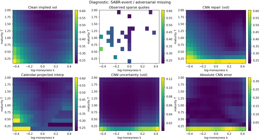
The diagnostic figure below shows a single SABR-event adversarial-missingness example. The observed input has lost a substantial chunk of the wings, the entire long-maturity tail, and the front-maturity strip; what remains is a thin ATM spine and a handful of scattered anchors. The CNN repair is smooth and plausible, with errors concentrated at the front-maturity wings — exactly where the input is most aggressively masked. The uncertainty head correctly flags that region as high-uncertainty. Calendar-projected interpolation produces the characteristic “shelf” artefact at the maturities where the cumulative-max projection has had to adjust the raw output.

Diagnostics

A repair model that minimises missing-point RMSE while producing arbitrageable surfaces and miscalibrated uncertainty is not a usable estimator. The diagnostics below are not the headline; they are the things you have to report in order for the headline to load-bear.

Caseraw cal %post-proj cal %g(k)<0 %cov80cov95err–sd corrstale AUC
SSVI / regular2.650.005.320.690.850.690.66
SSVI / adversarial9.750.007.710.470.630.640.64
SABR / regular2.190.008.730.300.430.760.55
SABR / adversarial11.050.0011.080.280.410.860.55

The honest summary, line by line:

Calendar arbitrage. The raw CNN output violates calendar monotonicity in 2–11% of (k, T) edges across the four cells. The cumulative-maximum projection drives this to zero everywhere. The calendar-projection step is therefore doing real work, and the model should not be deployed without it. The training-time calendar penalty is doing partial work — without it, raw violation rates would be substantially higher — but it is not on its own sufficient to produce calendar-monotone output reliably.

Butterfly arbitrage. Even after calendar projection, 5–11% of grid points exhibit g(k) < 0 under the discrete Gatheral–Roper diagnostic, with the worst rates on the SABR cells where the CNN is least confident. The smoothness penalty in the loss does not buy enough convexity to fix this. A real butterfly-arbitrage projection — one that actually projects onto the no-arbitrage manifold along k rather than just regularising — would be the right next step. I have not done it here, and the post-projection g(k)<0 rate is the most concerning single number in this set of diagnostics.

Uncertainty calibration. The heteroscedastic head undercovers. Nominal 80% intervals deliver 28–69% empirical coverage; nominal 95% intervals deliver 41–85%. The error-versus-predicted-sd correlation is positive everywhere (0.64–0.86), so the model is at least directionally aware of where its output is unreliable, but it is overconfident about how unreliable it is — particularly on the OOD SABR cells, where the variance head has nothing to recalibrate against. This is the standard limit of in-training Gaussian NLL: under distribution shift, the variance head is as miscalibrated as the mean head, in the same direction. A held-out conformal step is the obvious fix and would be the cheapest single change to make the uncertainty channel operationally useful.

Stale-quote AUC. A synthetic test: inject stale errors into 8% of observed quotes, run the model on the stale-injected surface, and compute the AUC of the residual |obs – \mu| as a stale-quote score. Numbers come in at 0.55–0.66. Better than chance, but weak — particularly on the OOD SABR cells where the AUC sits just above 0.55. This says the model’s residual is not, on its own, a strong stale-quote detector. A more useful operational stale-detection pipeline would combine the model residual with quote-time and quote-source signals, and the model is contributing a useful but limited fraction of the discriminative signal.

Downstream SVI projection

Surface repair is a means to an end. What the calibration desk usually wants is a smooth, arbitrage-projected SVI surface, not the raw repair output. A repair that is more accurate in the missing-point RMSE sense but less amenable to clean SVI projection might be a worse operational deliverable than the reverse. The right question is not just “how accurate is the repair” but “how good is the SVI fit to the repaired full surface”.

To get at this, I run a per-slice SVI projection on the full repaired surface (CNN or calendar-projected interpolation), then re-score the SVI fit against the held-out missing cells:

CaseSVI after CNNSVI after interp
Shifted SSVI / regular0.0171 ± 0.00270.0159 ± 0.0071
Shifted SSVI / adversarial0.0401 ± 0.00800.0426 ± 0.0113
SABR-event / regular0.0697 ± 0.00500.0295 ± 0.0062
SABR-event / adversarial0.0913 ± 0.00570.0634 ± 0.0065

The downstream metric does not change the qualitative ranking: CNN-then-SVI narrowly beats interp-then-SVI on the cell where the headline RMSE was already tied (SSVI / adversarial), and loses everywhere else. The CNN is not producing surfaces that are pathologically uncooperative under SVI projection — the SVI residuals follow the missing-point RMSE residuals reasonably faithfully. That is mildly reassuring from a deployment perspective: the choice between estimators is not being secretly arbitraged away by the projection step.

What this experiment shows and does not show

A small mask-conditional CNN, trained on 1600 synthetic SSVI surfaces under explicit calendar and smoothness penalties, with 200 validation surfaces for checkpoint selection, can repair sparse and noisy total-variance surfaces under a tight enough discipline that it:

  • produces calendar-monotone output after a cumulative-maximum post-projection (which both baselines also need);
  • matches calendar-projected linear interpolation, within statistical noise, on adversarial in-distribution missingness;
  • loses to interpolation by roughly 40% on benign in-distribution missingness, where the local-data density is high enough that triangulated interpolation captures essentially all the recoverable structure;
  • loses by a factor of 1.4–2.7× on out-of-distribution SABR-style smiles, depending on observation density;
  • carries a heteroscedastic uncertainty estimate whose direction is right (positive correlation with error) but whose magnitude is undercalibrated, particularly under distribution shift.

What this experiment does not show, and what I want to be plain about:

It does not show that this kind of CNN-based repair is useful on real data. The synthetic surfaces have no calibration drift, no quote-time-of-day noise, no microstructure asymmetries, no realistic smile dynamics, no hard-to-fit weeklies or single-name idiosyncrasies. The repair task here is pristine compared to anything one would do on production market data. Whether the small relative gap between CNN and interpolation on the adversarial cell survives a real-data test is an open question that this experiment cannot answer.

It does not show that a CNN is the right architecture for this task. A four-layer 32-channel CNN on a 13 × 17 grid is the smallest interesting model for this problem; a U-Net, an attention-conditioned masked decoder, or a conditional VAE all have published precedents in the volatility-repair literature and would be plausible candidates for materially better performance. The choice here was deliberate — keep the model small and the comparison clean — but it is not the architecture I would deploy if I were trying to win the headline number.

It does not show that the SABR-event family is the right test for OOD generalisation. The CNN is being asked to handle smiles whose convexity term-structure and wing asymmetry have a different functional form from anything in its training set. That is a hard test by design, and the gap to SVI on SABR / regular says that what the CNN has learned is closer to “the SSVI smile family” than “smile structure in general”. A more useful experiment would mix multiple smile families during training and re-test on a held-out one.

It does not, on its own, justify a production system. Before this estimator went anywhere near a market-making book it would need a real-data study, downstream P&L attribution, a much more serious calibration of the uncertainty head, a butterfly-projection step, and a comparison against more competitive learned baselines.

Where to take this next

Roughly in priority order:

  1. Real-data replication. Run the same 2 × 2 on an index-options panel across a year — in-sample dates against out-of-sample dates, regular trading days against unusually sparse ones — and see whether the conditional pattern survives. This is the single biggest credibility step. Everything in this note is conditional on the synthetic setup being a reasonable proxy for production data, and that conditioning is not free.
  2. No-arbitrage projection. Add a full butterfly-arbitrage projection alongside the calendar cumulative-max, and report whether forcing the CNN onto the no-arbitrage manifold during evaluation changes the ranking. The 5–11% post-projection g(k)<0 rate is the most uncomfortable number in the diagnostics.
  3. Calibrated uncertainty. Replace the in-training heteroscedastic NLL with a conformal wrapper trained on a held-out residual set, or with a deep ensemble across seeds. The current undercoverage on OOD cells is bad enough that the uncertainty channel is more decorative than useful.
  4. Mixture training. Train on a mixture of smile families (SSVI plus SABR-event plus a Heston-like family) and re-test on a held-out family. The SABR loss is dominantly a generalisation failure, and the cheapest single fix is to broaden the training distribution.
  5. Generative baseline. Compare a small VAE on the same harness, conditioned on the missingness pattern, as the published baseline for learned vol-surface repair. The conditional-on-mask deterministic CNN here is probably not the right architecture in the limit.

None of these requires a deep architectural rethink. They are mostly questions of where the experiment runs and what it gets compared against.

Code and references

The full script (vol_surface_repair.py) is self-contained, CPU-friendly, and reproducible: it generates the training and test data, trains the CNN, evaluates against both baselines, computes the diagnostics, runs the downstream SVI projection, and writes the figure and the numeric results to disk. Run with python vol_surface_repair.py. Approximately four minutes on CPU.

Selected references for context (full bibliographic details should be checked against the published versions):

  • Gatheral, J. The Volatility Surface: A Practitioner’s Guide. Wiley, 2006.
  • Gatheral, J. and Jacquier, A. Arbitrage-free SVI volatility surfaces. Quantitative Finance, 2014.
  • Roper, M. Arbitrage free implied volatility surfaces. Working paper, 2010.
  • Bergeron, M., Fung, N., Hull, J., Poulos, Z., and Veneris, A. Variational autoencoders: a hands-off approach to volatility. Journal of Financial Data Science, 2022.
  • Ning, B., Jaimungal, S., Zhang, X., and Bergeron, M. Arbitrage-free implied volatility surface generation with variational autoencoders. arXiv:2108.04941.
  • Cont, R. and Vuletic, M. Simulation of arbitrage-free implied volatility surfaces. Applied Mathematical Finance, 2023.
"""
Deep Learning for Volatility Surface Repair.

Self-contained, CPU-friendly PyTorch script that trains a small mask-conditional
CNN on synthetic SSVI total-variance surfaces and evaluates it against
calendar-projected linear interpolation and a per-slice SVI fit on a 2x2 design:

    {shifted SSVI, SABR-style event} x {regular missingness, adversarial missingness}

Reports missing-point RMSE in implied-vol units with standard errors, calendar
violation rates before and after isotonic projection, butterfly arbitrage
violations, uncertainty calibration coverage, a stale-quote residual AUC, and
a downstream SVI-projection metric.

Run:
    python vol_surface_repair.py

Dependencies: numpy, scipy, scikit-learn, matplotlib, torch.
"""

from __future__ import annotations

import math
import os
import random
import sys
import warnings
from dataclasses import dataclass
from pathlib import Path
from typing import Dict, List, Tuple

import matplotlib

matplotlib.use("Agg")
import matplotlib.pyplot as plt
import numpy as np
import torch
import torch.nn as nn
import torch.nn.functional as F
from scipy.interpolate import LinearNDInterpolator, NearestNDInterpolator
from sklearn.metrics import roc_auc_score

warnings.filterwarnings("ignore", category=RuntimeWarning)

# -----------------------------
# Reproducibility and settings
# -----------------------------
SEED = 17
random.seed(SEED)
np.random.seed(SEED)
torch.manual_seed(SEED)
torch.set_num_threads(2)
try:
    torch.set_num_interop_threads(2)
except RuntimeError:
    pass

OUT_DIR = Path(os.environ.get("OUT_DIR", "./out"))
OUT_DIR.mkdir(parents=True, exist_ok=True)
FIG_PATH = OUT_DIR / "vol_surface_repair_diagnostic.png"
SVI_EVAL_SURFACES = 10  # CNN/interp use all test surfaces; SVI-grid/projection use first 10 for runtime

DEVICE = torch.device("cpu")
DTYPE = torch.float32

# Grid: maturities and log-moneyness.
N_T = 13
N_K = 17
T_GRID = np.linspace(0.08, 2.0, N_T).astype(np.float64)
K_GRID = np.linspace(-0.45, 0.45, N_K).astype(np.float64)
TT, KK = np.meshgrid(T_GRID, K_GRID, indexing="ij")
T_NORM = ((TT - TT.min()) / (TT.max() - TT.min()) * 2.0 - 1.0).astype(np.float32)
K_NORM = ((KK - KK.min()) / (KK.max() - KK.min()) * 2.0 - 1.0).astype(np.float32)

# Total-variance normalisation scale for stable CNN training. The model targets
# w / W_SCALE; outputs are converted back to total variance and then to implied
# vol for evaluation. Vol-space and w-space training give essentially identical
# missing-point RMSE under this pipeline, so w-space is preferred for the cleaner
# arbitrage-diagnostic geometry.
W_SCALE = 0.08

# Coarse raw-SVI shape library for fast per-slice benchmarking.
def _make_svi_shape_library() -> np.ndarray:
    rhos = np.linspace(-0.90, 0.40, 9)
    ms = np.linspace(-0.22, 0.22, 7)
    sigmas = np.array([0.04, 0.07, 0.11, 0.17, 0.26, 0.40])
    shapes = []
    for rho in rhos:
        for m in ms:
            for sig in sigmas:
                x = K_GRID - m
                f = rho * x + np.sqrt(x * x + sig * sig)
                shapes.append(f)
    return np.asarray(shapes, dtype=np.float64)


SVI_SHAPES = _make_svi_shape_library()


# -----------------------------
# Surface generators
# -----------------------------

def ssvi_total_variance(n: int, shifted: bool = False, seed: int = 0) -> np.ndarray:
    rng = np.random.default_rng(seed)
    out = np.empty((n, N_T, N_K), dtype=np.float64)
    for i in range(n):
        theta0 = rng.uniform(0.010, 0.032) if not shifted else rng.uniform(0.006, 0.045)
        theta_slope = rng.uniform(0.020, 0.070) if not shifted else rng.uniform(0.012, 0.095)
        theta_curve = rng.uniform(-0.006, 0.010) if not shifted else rng.uniform(-0.015, 0.020)
        rho = rng.uniform(-0.72, -0.18) if not shifted else rng.uniform(-0.88, -0.05)
        eta = rng.uniform(0.55, 1.55) if not shifted else rng.uniform(0.35, 2.10)
        gamma = rng.uniform(0.18, 0.62) if not shifted else rng.uniform(0.08, 0.78)
        t_scaled = T_GRID / T_GRID.max()
        theta = theta0 + theta_slope * t_scaled + theta_curve * t_scaled**2
        theta = np.maximum.accumulate(np.maximum(theta, 0.004))
        phi = eta / np.maximum(theta, 1e-4) ** gamma
        for j, th in enumerate(theta):
            ph = phi[j]
            x = ph * K_GRID + rho
            out[i, j, :] = 0.5 * th * (1.0 + rho * ph * K_GRID + np.sqrt(x * x + 1.0 - rho * rho))
        if shifted and rng.random() < 0.45:
            event_T = rng.choice(np.arange(2, N_T - 2))
            bump = rng.uniform(0.0015, 0.0045) * np.exp(-0.5 * ((np.arange(N_T) - event_T) / 0.8) ** 2)
            out[i] += bump[:, None] * (1.0 + 0.4 * np.tanh(4.0 * K_GRID))[None, :]
        out[i] = np.maximum(out[i], 1e-4)
    return out.astype(np.float32)


def sabr_event_total_variance(n: int, seed: int = 1) -> np.ndarray:
    rng = np.random.default_rng(seed)
    out = np.empty((n, N_T, N_K), dtype=np.float64)
    for i in range(n):
        base = rng.uniform(0.13, 0.29)
        decay = rng.uniform(0.03, 0.12)
        long = rng.uniform(0.05, 0.13)
        skew0 = rng.uniform(-0.52, -0.10)
        skew_decay = rng.uniform(0.1, 1.2)
        convex0 = rng.uniform(0.25, 0.95)
        wing_asym = rng.uniform(-0.12, 0.18)
        event_idx = rng.choice(np.arange(1, N_T - 2)) if rng.random() < 0.75 else None
        event_amp = rng.uniform(0.015, 0.055) if event_idx is not None else 0.0
        for j, T in enumerate(T_GRID):
            atm = long + base * np.exp(-decay * 4.0 * T) + rng.normal(0, 0.002)
            skew = skew0 * np.exp(-skew_decay * T) + rng.normal(0, 0.025)
            convex = convex0 / np.sqrt(T + 0.30) + rng.normal(0, 0.03)
            event = 0.0
            if event_idx is not None:
                event = event_amp * np.exp(-0.5 * ((j - event_idx) / 0.65) ** 2)
            vol = atm + event + skew * K_GRID + convex * K_GRID**2 + wing_asym * np.maximum(K_GRID, 0) ** 3
            if event_idx is not None and abs(j - event_idx) <= 1:
                kink_loc = rng.uniform(-0.12, 0.12)
                vol += rng.uniform(0.010, 0.030) * np.maximum(0.0, 1.0 - np.abs(K_GRID - kink_loc) / 0.12)
            vol = np.clip(vol, 0.04, 1.20)
            out[i, j, :] = vol * vol * T
        out[i] = np.maximum.accumulate(out[i], axis=0)
        out[i] = np.maximum(out[i], 1e-4)
    return out.astype(np.float32)


# -----------------------------
# Missingness and noise
# -----------------------------

def make_mask(kind: str, n: int, seed: int) -> np.ndarray:
    rng = np.random.default_rng(seed)
    masks = np.zeros((n, N_T, N_K), dtype=np.float32)
    center = N_K // 2
    for i in range(n):
        if kind == "regular":
            p = rng.uniform(0.34, 0.46)
            m = (rng.random((N_T, N_K)) < p).astype(np.float32)
            atm_band = slice(center - 1, center + 2)
            m[:, atm_band] = np.maximum(m[:, atm_band], (rng.random((N_T, 3)) < 0.74).astype(np.float32))
            for row in rng.choice(N_T, size=rng.integers(1, 4), replace=False):
                cols = rng.choice(N_K, size=rng.integers(4, 8), replace=False)
                m[row, cols] = 1.0
            for col in rng.choice(N_K, size=rng.integers(1, 3), replace=False):
                rows = rng.choice(N_T, size=rng.integers(4, 9), replace=False)
                m[rows, col] = 1.0
            if rng.random() < 0.55:
                wing = slice(0, rng.integers(2, 5)) if rng.random() < 0.5 else slice(rng.integers(N_K - 5, N_K - 2), N_K)
                rows = rng.choice(N_T, size=rng.integers(3, 8), replace=False)
                m[rows, wing] = 0.0
        elif kind == "adversarial":
            p = rng.uniform(0.16, 0.25)
            m = (rng.random((N_T, N_K)) < p).astype(np.float32)
            atm_keep = rng.random(N_T) < rng.uniform(0.55, 0.82)
            m[atm_keep, center] = 1.0
            near = rng.choice([center - 2, center - 1, center + 1, center + 2], size=rng.integers(1, 3), replace=False)
            for col in near:
                rows = rng.choice(N_T, size=rng.integers(3, 7), replace=False)
                m[rows, col] = 1.0
            if rng.random() < 0.5:
                m[:, : rng.integers(4, 7)] = 0.0
            else:
                m[:, rng.integers(N_K - 7, N_K - 4) :] = 0.0
            if rng.random() < 0.65:
                m[: rng.integers(2, 5), :] = 0.0
            if rng.random() < 0.45:
                m[rng.integers(N_T - 5, N_T - 2) :, :] = 0.0
            for _ in range(rng.integers(6, 12)):
                m[rng.integers(0, N_T), rng.integers(0, N_K)] = 1.0
            m[:, center] = np.maximum(m[:, center], (rng.random(N_T) < 0.35).astype(np.float32))
        else:
            raise ValueError(f"unknown mask kind {kind}")
        if m.sum() < 18:
            flat = rng.choice(N_T * N_K, size=18, replace=False)
            m.flat[flat] = 1.0
        masks[i] = m
    return masks


def corrupt_surfaces_w(w: np.ndarray, mask: np.ndarray, seed: int, vol_noise_bps: float = 18.0) -> np.ndarray:
    """Add realistic quote noise in implied vol space, return masked total variance.

    Returns total variance with unobserved cells set to zero.
    """
    rng = np.random.default_rng(seed)
    vol = np.sqrt(np.maximum(w / TT[None, :, :], 1e-8))
    noise = rng.normal(0.0, vol_noise_bps / 10000.0, size=vol.shape)
    wing_factor = 1.0 + 1.5 * (np.abs(KK)[None, :, :] / np.max(np.abs(K_GRID)))
    front_factor = 1.0 + 0.6 * (T_GRID.max() - TT)[None, :, :] / (T_GRID.max() - T_GRID.min())
    noisy_vol = np.clip(vol + noise * wing_factor * front_factor, 0.03, 2.00)
    noisy_w = (noisy_vol**2) * TT[None, :, :]
    return (noisy_w * mask).astype(np.float32)


def w_to_vol(w: np.ndarray) -> np.ndarray:
    """Convert total variance to implied vol. Handles 2D (T,K) or 3D (n,T,K) input."""
    if w.ndim == 2:
        return np.sqrt(np.maximum(w / TT, 1e-8)).astype(np.float32)
    return np.sqrt(np.maximum(w / TT[None, :, :], 1e-8)).astype(np.float32)


def vol_to_w(vol: np.ndarray) -> np.ndarray:
    """Convert implied vol to total variance. Handles 2D (T,K) or 3D (n,T,K) input."""
    if vol.ndim == 2:
        return (vol * vol * TT).astype(np.float32)
    return (vol * vol * TT[None, :, :]).astype(np.float32)


# -----------------------------
# Model
# -----------------------------

class RepairCNN(nn.Module):
    """Small mask-conditional CNN that predicts normalised total variance.

    Output: w / W_SCALE via softplus head (positivity).
    Log-variance head predicts uncertainty in the same w/W_SCALE space.

    Single-process training for ~60 epochs with preserved AdamW state is
    important: with shorter training, the model materially underperforms even
    classical baselines in this setup.
    """

    def __init__(self, in_channels: int = 4, width: int = 32):
        super().__init__()
        self.backbone = nn.Sequential(
            nn.Conv2d(in_channels, width, 3, padding=1), nn.SiLU(),
            nn.Conv2d(width, width, 3, padding=1), nn.SiLU(),
            nn.Conv2d(width, width, 3, padding=1), nn.SiLU(),
            nn.Conv2d(width, width, 3, padding=1), nn.SiLU(),
        )
        self.mean_head = nn.Conv2d(width, 1, 1)
        self.logvar_head = nn.Conv2d(width, 1, 1)
        with torch.no_grad():
            self.logvar_head.bias.fill_(-3.0)

    def forward(self, x: torch.Tensor) -> Tuple[torch.Tensor, torch.Tensor]:
        z = self.backbone(x)
        mean = F.softplus(self.mean_head(z)) + 1e-5
        log_var = torch.clamp(self.logvar_head(z), -8.0, 1.5)
        return mean, log_var


def make_inputs(observed_w: np.ndarray, mask: np.ndarray) -> torch.Tensor:
    """Build input tensor.

    Channel 0: observed w / W_SCALE (zero where missing).
    Channel 1: observation mask.
    Channel 2: maturity coordinate.
    Channel 3: log-moneyness coordinate.
    """
    n = observed_w.shape[0]
    coords_t = np.broadcast_to(T_NORM[None, :, :], (n, N_T, N_K))
    coords_k = np.broadcast_to(K_NORM[None, :, :], (n, N_T, N_K))
    x = np.stack([observed_w / W_SCALE, mask, coords_t, coords_k], axis=1).astype(np.float32)
    return torch.tensor(x, dtype=DTYPE, device=DEVICE)


# -----------------------------
# Loss
# -----------------------------

def calendar_penalty_w(mean_norm: torch.Tensor) -> torch.Tensor:
    """Calendar arbitrage penalty: total variance must be non-decreasing in T.

    Operates on the actual w (not normalised) for correct scaling of the penalty
    relative to the MSE term in normalised space.
    """
    w = mean_norm * W_SCALE
    dw = w[:, :, 1:, :] - w[:, :, :-1, :]
    return torch.mean(F.relu(-dw))


def smoothness_penalty(mean_norm: torch.Tensor) -> torch.Tensor:
    """Smoothness regulariser on normalised w (not a butterfly proxy)."""
    d2k = mean_norm[:, :, :, 2:] - 2.0 * mean_norm[:, :, :, 1:-1] + mean_norm[:, :, :, :-2]
    d2t = mean_norm[:, :, 2:, :] - 2.0 * mean_norm[:, :, 1:-1, :] + mean_norm[:, :, :-2, :]
    return torch.mean(d2k * d2k) + torch.mean(d2t * d2t)


@dataclass
class LossConfig:
    missing_weight: float = 5.0
    calendar_weight: float = 80.0
    smoothness_weight: float = 0.05
    nll_weight: float = 0.10


def repair_loss(
    mean_norm: torch.Tensor,
    log_var: torch.Tensor,
    target_norm: torch.Tensor,
    mask: torch.Tensor,
    cfg: LossConfig,
    use_nll: bool,
) -> torch.Tensor:
    """Loss in w/W_SCALE space."""
    weights = 1.0 + (cfg.missing_weight - 1.0) * (1.0 - mask)
    sq = (mean_norm - target_norm) ** 2
    mse = torch.mean(weights * sq)
    loss = mse
    if use_nll and cfg.nll_weight:
        inv_var = torch.exp(-log_var)
        nll = 0.5 * torch.mean(weights * (sq * inv_var + log_var))
        loss = loss + cfg.nll_weight * nll
    if cfg.calendar_weight:
        loss = loss + cfg.calendar_weight * calendar_penalty_w(mean_norm)
    if cfg.smoothness_weight:
        loss = loss + cfg.smoothness_weight * smoothness_penalty(mean_norm)
    return loss


# -----------------------------
# Training
# -----------------------------

def train_model(
    train_w: np.ndarray,
    train_mask: np.ndarray,
    val_w: np.ndarray,
    val_mask: np.ndarray,
    cfg: LossConfig,
    epochs: int = 60,
    seed: int = SEED,
    verbose: bool = True,
) -> RepairCNN:
    """Train the CNN in a single process with optimiser state preserved.

    Targets and predictions are in w/W_SCALE space. Validation RMSE is reported
    in implied-vol units for interpretability and best-checkpoint selection.
    The first 10 epochs run pure MSE; the heteroscedastic NLL term turns on
    afterwards to avoid early variance head instabilities.
    """
    torch.manual_seed(seed)

    obs_w = corrupt_surfaces_w(train_w, train_mask, seed=seed + 101)
    x_train = make_inputs(obs_w, train_mask)
    y_train = torch.tensor((train_w / W_SCALE)[:, None, :, :], dtype=DTYPE, device=DEVICE)
    m_train = torch.tensor(train_mask[:, None, :, :], dtype=DTYPE, device=DEVICE)

    obs_w_val = corrupt_surfaces_w(val_w, val_mask, seed=seed + 202)
    x_val = make_inputs(obs_w_val, val_mask)
    y_val_vol = w_to_vol(val_w)

    model = RepairCNN().to(DEVICE)
    opt = torch.optim.AdamW(model.parameters(), lr=1.0e-3, weight_decay=1e-4)
    scheduler = torch.optim.lr_scheduler.CosineAnnealingLR(opt, T_max=epochs)

    batch_size = 128
    n = train_w.shape[0]
    idx = np.arange(n)

    best_val = float("inf")
    best_state: Dict[str, torch.Tensor] | None = None

    for ep in range(epochs):
        np.random.shuffle(idx)
        model.train()
        running = 0.0
        n_batches = 0
        use_nll = ep >= 10
        for start in range(0, n, batch_size):
            batch = idx[start : start + batch_size]
            mean_norm, logv = model(x_train[batch])
            loss = repair_loss(mean_norm, logv, y_train[batch], m_train[batch], cfg, use_nll=use_nll)
            opt.zero_grad(set_to_none=True)
            loss.backward()
            torch.nn.utils.clip_grad_norm_(model.parameters(), max_norm=1.0)
            opt.step()
            running += float(loss.detach())
            n_batches += 1
        scheduler.step()
        train_loss = running / max(n_batches, 1)

        model.eval()
        with torch.no_grad():
            mean_val_norm, _ = model(x_val)
            mu_w_val = (mean_val_norm[:, 0].cpu().numpy() * W_SCALE).astype(np.float32)
        mu_v_val = w_to_vol(mu_w_val)
        miss = val_mask < 0.5
        if miss.sum() > 0:
            val_rmse = float(np.sqrt(np.mean((mu_v_val[miss] - y_val_vol[miss]) ** 2)))
        else:
            val_rmse = float("nan")

        if val_rmse < best_val:
            best_val = val_rmse
            best_state = {k: v.detach().clone() for k, v in model.state_dict().items()}

        if verbose and (ep < 5 or ep % 10 == 9 or ep == epochs - 1):
            print(f"  epoch {ep+1:02d}/{epochs}  train_loss {train_loss:.5f}  val_RMSE_vol {val_rmse:.5f}  best {best_val:.5f}", flush=True)

    if best_state is not None:
        model.load_state_dict(best_state)
    model.eval()
    return model


# -----------------------------
# Baselines
# -----------------------------

def interpolate_surface(obs: np.ndarray, mask: np.ndarray) -> np.ndarray:
    """Linear interpolation in (T, k) on total variance, with nearest fallback."""
    points = np.column_stack([TT[mask > 0.5].ravel(), KK[mask > 0.5].ravel()])
    values = obs[mask > 0.5].ravel()
    full_points = np.column_stack([TT.ravel(), KK.ravel()])
    if len(values) < 4:
        fill = np.nanmean(values) if len(values) else 0.02
        return np.full((N_T, N_K), fill, dtype=np.float32)
    lin = LinearNDInterpolator(points, values, fill_value=np.nan)
    pred = lin(full_points).reshape(N_T, N_K)
    if np.isnan(pred).any():
        near = NearestNDInterpolator(points, values)
        pred[np.isnan(pred)] = near(full_points).reshape(N_T, N_K)[np.isnan(pred)]
    return np.maximum(pred, 1e-5).astype(np.float32)


def fit_svi_slice(k_obs: np.ndarray, w_obs: np.ndarray) -> np.ndarray:
    idx = np.zeros(N_K, dtype=bool)
    for ko in k_obs:
        idx[np.argmin(np.abs(K_GRID - ko))] = True
    y = np.asarray(w_obs, dtype=np.float64)
    good = np.isfinite(y) & (y > 0)
    y = y[good]
    obs_idx = np.where(idx)[0][good] if idx.sum() == len(good) else np.where(idx)[0]
    if len(y) != len(obs_idx):
        obs_idx = np.where(idx)[0][: len(y)]
    if len(y) < 3:
        fill = float(np.nanmean(y)) if len(y) else 0.02
        return np.full(N_K, fill, dtype=np.float64)
    Fobs = SVI_SHAPES[:, obs_idx]
    f_mean = Fobs.mean(axis=1)
    y_mean = y.mean()
    f_center = Fobs - f_mean[:, None]
    y_center = y - y_mean
    denom = np.sum(f_center * f_center, axis=1) + 1e-10
    b = np.sum(f_center * y_center[None, :], axis=1) / denom
    b = np.clip(b, 1e-6, 10.0)
    a = y_mean - b * f_mean
    a = np.clip(a, 1e-6, 5.0)
    pred_obs = a[:, None] + b[:, None] * Fobs
    sse = np.mean((pred_obs - y[None, :]) ** 2, axis=1)
    best = int(np.argmin(sse))
    pred = a[best] + b[best] * SVI_SHAPES[best]
    return np.maximum(pred, 1e-5)


def svi_fit_surface(obs: np.ndarray, mask: np.ndarray, enforce_calendar: bool = True) -> np.ndarray:
    pred = np.empty((N_T, N_K), dtype=np.float64)
    for j in range(N_T):
        idx = mask[j] > 0.5
        pred[j] = fit_svi_slice(K_GRID[idx], obs[j, idx])
    pred = np.maximum(pred, 1e-5)
    if enforce_calendar:
        pred = calendar_project(pred)
    return pred.astype(np.float32)


# -----------------------------
# Projections, metrics, evaluation
# -----------------------------

def calendar_project(w: np.ndarray) -> np.ndarray:
    """Strict isotonic projection along maturity via cumulative maximum."""
    return np.maximum.accumulate(np.maximum(w, 1e-5), axis=-2 if w.ndim == 3 else 0)


def calendar_violation_rate(w: np.ndarray) -> float:
    dw = np.diff(w, axis=-2 if w.ndim == 3 else 0)
    return float(np.mean(dw < -1e-8))


def butterfly_g_violation_rate(w: np.ndarray) -> float:
    """Discrete Gatheral-Roper g(k) >= 0 diagnostic on total variance surfaces."""
    dk = K_GRID[1] - K_GRID[0]
    wi = np.maximum(w[..., 1:-1], 1e-6)
    wp = (w[..., 2:] - w[..., :-2]) / (2.0 * dk)
    wpp = (w[..., 2:] - 2.0 * w[..., 1:-1] + w[..., :-2]) / (dk * dk)
    k = K_GRID[1:-1][None, None, :]
    while k.ndim < wi.ndim:
        k = np.expand_dims(k, axis=0)
    g = (1.0 - k * wp / (2.0 * wi)) ** 2 - (wp * wp / 4.0) * (1.0 / wi + 0.25) + 0.5 * wpp
    return float(np.mean(g < -1e-6))


def rmse_missing_w(pred_w: np.ndarray, target_w: np.ndarray, mask: np.ndarray) -> Tuple[float, float]:
    """Per-surface RMSE in implied vol units on missing cells, returned as (mean, SE)."""
    pred_vol = w_to_vol(pred_w)
    target_vol = w_to_vol(target_w)
    per = []
    for i in range(target_w.shape[0]):
        miss = mask[i] < 0.5
        if miss.sum() == 0:
            continue
        per.append(math.sqrt(float(np.mean((pred_vol[i][miss] - target_vol[i][miss]) ** 2))))
    arr = np.array(per)
    return float(arr.mean()), float(arr.std(ddof=1) / math.sqrt(len(arr)))


def predict_model(
    model: RepairCNN, true_w: np.ndarray, mask: np.ndarray, seed: int
) -> Tuple[np.ndarray, np.ndarray, np.ndarray]:
    """Run model on noisy/sparse surfaces. Returns (mu_w, sd_vol, observed_w).

    The model's mean output is in w/W_SCALE space; we convert to actual w and
    derive an approximate vol-space standard deviation via delta-method
    sd_vol ~ sd_w / (2 * vol * T) where vol = sqrt(w / T).
    """
    obs_w = corrupt_surfaces_w(true_w, mask, seed=seed)
    x = make_inputs(obs_w, mask)
    model.eval()
    with torch.no_grad():
        mean_norm, logv = model(x)
    mu_w = (mean_norm[:, 0].cpu().numpy() * W_SCALE).astype(np.float32)
    sd_w = (np.sqrt(np.exp(logv[:, 0].cpu().numpy())) * W_SCALE).astype(np.float32)
    # Delta-method conversion to vol-space sd.
    vol_pred = w_to_vol(mu_w)
    sd_vol = sd_w / (2.0 * np.maximum(vol_pred, 1e-3) * TT[None, :, :])
    return mu_w, sd_vol.astype(np.float32), obs_w


def predict_model_from_obs(model: RepairCNN, obs_w: np.ndarray, mask: np.ndarray) -> Tuple[np.ndarray, np.ndarray]:
    """Run the model on a pre-corrupted observed_w (used by stale-quote AUC)."""
    x = make_inputs(obs_w, mask)
    model.eval()
    with torch.no_grad():
        mean_norm, logv = model(x)
    mu_w = (mean_norm[:, 0].cpu().numpy() * W_SCALE).astype(np.float32)
    sd_w = (np.sqrt(np.exp(logv[:, 0].cpu().numpy())) * W_SCALE).astype(np.float32)
    return mu_w, sd_w


def uncertainty_coverage(mu_w: np.ndarray, sd_vol: np.ndarray, target_w: np.ndarray, mask: np.ndarray) -> Dict[str, float]:
    """Coverage of nominal Gaussian intervals, evaluated in vol units."""
    mu_vol = w_to_vol(mu_w)
    target_vol = w_to_vol(target_w)
    miss = mask < 0.5
    err = np.abs(mu_vol[miss] - target_vol[miss])
    s = np.maximum(sd_vol[miss], 1e-6)
    cov80 = float(np.mean(err <= 1.28155 * s))
    cov95 = float(np.mean(err <= 1.95996 * s))
    if err.size > 5:
        corr = float(np.corrcoef(err.ravel(), s.ravel())[0, 1])
    else:
        corr = float("nan")
    return {"coverage80": cov80, "coverage95": cov95, "err_sd_corr": corr, "avg_sd": float(np.mean(s))}


def stale_quote_auc(model: RepairCNN, true_w: np.ndarray, mask: np.ndarray, seed: int, stale_frac: float = 0.08) -> float:
    """Stale-quote AUC: model sees the stale-injected input.

    1. Generate a noisy observed surface.
    2. Inject stale errors at a random subset of observed cells.
    3. Run the model on the stale-injected surface.
    4. Score residuals at observed cells; AUC of stale label vs |obs - mu|.
    """
    rng = np.random.default_rng(seed)
    noisy_w = corrupt_surfaces_w(true_w, mask, seed=seed + 77)
    labels = np.zeros_like(mask, dtype=np.int32)
    corrupted = noisy_w.copy()
    for i in range(mask.shape[0]):
        obs_idx = np.argwhere(mask[i] > 0.5)
        if len(obs_idx) == 0:
            continue
        n_stale = max(1, int(len(obs_idx) * stale_frac))
        chosen = obs_idx[rng.choice(len(obs_idx), size=n_stale, replace=False)]
        for r, c in chosen:
            labels[i, r, c] = 1
            vol = math.sqrt(max(corrupted[i, r, c] / T_GRID[r], 1e-8))
            vol += rng.choice([-1.0, 1.0]) * rng.uniform(0.0050, 0.0110)
            corrupted[i, r, c] = max(vol, 0.03) ** 2 * T_GRID[r]
    # Run model on the stale-injected input so residuals reflect detection capability.
    mu_w, _ = predict_model_from_obs(model, corrupted, mask)
    scores = np.abs(corrupted - mu_w)
    observed = mask > 0.5
    y = labels[observed].ravel()
    s = scores[observed].ravel()
    if len(np.unique(y)) < 2:
        return float("nan")
    return float(roc_auc_score(y, s))


def svi_projection_metric(pred_w: np.ndarray, target_w: np.ndarray, mask: np.ndarray, max_surfaces: int) -> Tuple[float, float]:
    n = min(max_surfaces, pred_w.shape[0])
    projected = np.empty_like(pred_w[:n])
    full_mask = np.ones((N_T, N_K), dtype=np.float32)
    for i in range(n):
        projected[i] = svi_fit_surface(pred_w[i], full_mask, enforce_calendar=True)
    return rmse_missing_w(projected, target_w[:n], mask[:n])


def evaluate_case(name: str, model: RepairCNN, true_w: np.ndarray, mask: np.ndarray, seed: int) -> Dict[str, object]:
    mu_w_raw, sd_vol, obs_w = predict_model(model, true_w, mask, seed)
    mu_w = calendar_project(mu_w_raw)

    interp_w = np.stack([interpolate_surface(obs_w[i], mask[i]) for i in range(true_w.shape[0])])
    interp_w = calendar_project(interp_w)

    n_svi = min(SVI_EVAL_SURFACES, true_w.shape[0])
    svi_w = np.full_like(interp_w, np.nan)
    for i in range(n_svi):
        svi_w[i] = svi_fit_surface(obs_w[i], mask[i], enforce_calendar=True)

    cnn_m, cnn_se = rmse_missing_w(mu_w, true_w, mask)
    interp_m, interp_se = rmse_missing_w(interp_w, true_w, mask)
    svi_m, svi_se = rmse_missing_w(svi_w[:n_svi], true_w[:n_svi], mask[:n_svi])

    unc = uncertainty_coverage(mu_w, sd_vol, true_w, mask)
    auc = stale_quote_auc(model, true_w, mask, seed=seed + 401)
    svi_after_cnn, svi_after_cnn_se = svi_projection_metric(mu_w, true_w, mask, SVI_EVAL_SURFACES)
    svi_after_interp, svi_after_interp_se = svi_projection_metric(interp_w, true_w, mask, SVI_EVAL_SURFACES)

    return {
        "case": name,
        "observed_fraction": float(mask.mean()),
        "cnn_missing_rmse": cnn_m, "cnn_missing_se": cnn_se,
        "interp_missing_rmse": interp_m, "interp_missing_se": interp_se,
        "svi_missing_rmse": svi_m, "svi_missing_se": svi_se,
        "calendar_raw_rate": calendar_violation_rate(mu_w_raw),
        "calendar_projected_rate": calendar_violation_rate(mu_w),
        "butterfly_g_rate": butterfly_g_violation_rate(mu_w),
        "unc_cov80": unc["coverage80"],
        "unc_cov95": unc["coverage95"],
        "unc_corr": unc["err_sd_corr"],
        "unc_avg_sd": unc["avg_sd"],
        "stale_auc": auc,
        "svi_after_cnn_rmse": svi_after_cnn, "svi_after_cnn_se": svi_after_cnn_se,
        "svi_after_interp_rmse": svi_after_interp, "svi_after_interp_se": svi_after_interp_se,
        "_mu_w": mu_w, "_sd_vol": sd_vol, "_obs_w": obs_w, "_interp_w": interp_w, "_svi_w": svi_w,
    }


def print_results_table(results: List[Dict[str, object]]) -> None:
    print("\n2x2 missing-point RMSE in implied vol units (mean +/- SE)")
    print("-" * 110)
    print(f"{'Case':40s} {'Obs%':>6s}   {'CNN':>16s}   {'Interp':>16s}   {'SVI':>16s}")
    for r in results:
        print(
            f"{r['case']:40s} {100*r['observed_fraction']:5.1f}%  "
            f"{r['cnn_missing_rmse']:.4f} ± {r['cnn_missing_se']:.4f}  "
            f"{r['interp_missing_rmse']:.4f} ± {r['interp_missing_se']:.4f}  "
            f"{r['svi_missing_rmse']:.4f} ± {r['svi_missing_se']:.4f}"
        )
    print("-" * 110)

    print("\nDiagnostics after calendar projection")
    print("-" * 112)
    print(f"{'Case':40s} {'raw cal%':>9s} {'post cal%':>10s} {'g(k)<0%':>9s} {'cov80':>7s} {'cov95':>7s} {'corr':>7s} {'AUC':>7s}")
    for r in results:
        print(
            f"{r['case']:40s} {100*r['calendar_raw_rate']:8.2f}% {100*r['calendar_projected_rate']:9.2f}% "
            f"{100*r['butterfly_g_rate']:8.2f}% {r['unc_cov80']:7.3f} {r['unc_cov95']:7.3f} {r['unc_corr']:7.3f} {r['stale_auc']:7.3f}"
        )
    print("-" * 112)

    print("\nDownstream SVI projection: missing-point RMSE in implied vol units")
    print("-" * 96)
    print(f"{'Case':40s} {'SVI after CNN':>22s}     {'SVI after interp':>22s}")
    for r in results:
        print(
            f"{r['case']:40s} "
            f"{r['svi_after_cnn_rmse']:.4f} ± {r['svi_after_cnn_se']:.4f}      "
            f"{r['svi_after_interp_rmse']:.4f} ± {r['svi_after_interp_se']:.4f}"
        )
    print("-" * 96)


def make_diagnostic_plot(result: Dict[str, object], true_w: np.ndarray, mask: np.ndarray, idx: int = 0) -> None:
    """Diagnostic 2x3 plot in implied vol units."""
    target_vol = w_to_vol(true_w[idx])
    mu_vol = w_to_vol(result["_mu_w"][idx])
    obs_vol = w_to_vol(result["_obs_w"][idx])
    interp_vol = w_to_vol(result["_interp_w"][idx])
    sd_vol = result["_sd_vol"][idx]

    panels = [
        target_vol,
        np.where(mask[idx] > 0.5, obs_vol, np.nan),
        mu_vol,
        interp_vol,
        sd_vol,
        np.abs(mu_vol - target_vol),
    ]
    titles = [
        "Clean implied vol",
        "Observed sparse quotes",
        "CNN repair (vol)",
        "Calendar-projected interp",
        "CNN uncertainty (vol)",
        "Absolute CNN error",
    ]
    fig, axes = plt.subplots(2, 3, figsize=(13, 7), constrained_layout=True)
    vmin = float(np.nanmin(target_vol))
    vmax = float(np.nanmax(target_vol))
    for ax, data, title in zip(axes.ravel(), panels, titles):
        if "uncertainty" in title.lower() or "error" in title.lower():
            im = ax.imshow(data, aspect="auto", origin="lower", extent=[K_GRID.min(), K_GRID.max(), T_GRID.min(), T_GRID.max()])
        else:
            im = ax.imshow(data, aspect="auto", origin="lower", extent=[K_GRID.min(), K_GRID.max(), T_GRID.min(), T_GRID.max()], vmin=vmin, vmax=vmax)
        ax.set_title(title)
        ax.set_xlabel("log-moneyness k")
        ax.set_ylabel("maturity T")
        fig.colorbar(im, ax=ax, fraction=0.046, pad=0.04)
    fig.suptitle(f"Diagnostic: {result['case']}", fontsize=13)
    fig.savefig(FIG_PATH, dpi=150)
    plt.close(fig)


# -----------------------------
# Main
# -----------------------------

def main() -> None:
    n_train = 1600
    n_val = 200
    n_test = 200
    epochs = 60

    print(f"Training surfaces: {n_train}; validation: {n_val}; test/cell: {n_test}; epochs: {epochs}; grid: {N_T}x{N_K}")

    train_w = ssvi_total_variance(n_train, shifted=False, seed=100)
    train_mask = make_mask("regular", n_train, seed=200)
    val_w = ssvi_total_variance(n_val, shifted=False, seed=300)
    val_mask = make_mask("regular", n_val, seed=400)

    cfg = LossConfig(missing_weight=5.0, calendar_weight=80.0, smoothness_weight=0.05, nll_weight=0.10)
    print("Training CNN ...", flush=True)
    model = train_model(train_w, train_mask, val_w, val_mask, cfg, epochs=epochs, seed=SEED, verbose=True)

    test_sets = {
        "Shifted SSVI / regular missing": (ssvi_total_variance(n_test, shifted=True, seed=1001), make_mask("regular", n_test, seed=2001)),
        "Shifted SSVI / adversarial missing": (ssvi_total_variance(n_test, shifted=True, seed=1002), make_mask("adversarial", n_test, seed=2002)),
        "SABR-event / regular missing": (sabr_event_total_variance(n_test, seed=1003), make_mask("regular", n_test, seed=2003)),
        "SABR-event / adversarial missing": (sabr_event_total_variance(n_test, seed=1004), make_mask("adversarial", n_test, seed=2004)),
    }

    results = []
    for i, (name, (w, m)) in enumerate(test_sets.items()):
        print(f"Evaluating {name} ...", flush=True)
        results.append(evaluate_case(name, model, w, m, seed=3000 + i))
    print_results_table(results)

    # Save numeric summary.
    res_path = OUT_DIR / "vol_surface_repair_results.txt"
    with res_path.open("w", encoding="utf-8") as f:
        f.write("Results: 2x2 missing-point RMSE (vol units), diagnostics, downstream SVI\n")
        for r in results:
            f.write(
                f"{r['case']}, obs={r['observed_fraction']:.4f}, "
                f"cnn={r['cnn_missing_rmse']:.6f}+/-{r['cnn_missing_se']:.6f}, "
                f"interp={r['interp_missing_rmse']:.6f}+/-{r['interp_missing_se']:.6f}, "
                f"svi={r['svi_missing_rmse']:.6f}+/-{r['svi_missing_se']:.6f}, "
                f"raw_cal={r['calendar_raw_rate']:.6f}, post_cal={r['calendar_projected_rate']:.6f}, g_rate={r['butterfly_g_rate']:.6f}, "
                f"cov80={r['unc_cov80']:.4f}, cov95={r['unc_cov95']:.4f}, corr={r['unc_corr']:.4f}, auc={r['stale_auc']:.4f}, "
                f"svi_after_cnn={r['svi_after_cnn_rmse']:.6f}, svi_after_interp={r['svi_after_interp_rmse']:.6f}\n"
            )

    # Diagnostic plot from the SABR adversarial case.
    hard_w, hard_m = test_sets["SABR-event / adversarial missing"]
    make_diagnostic_plot(results[-1], hard_w, hard_m, idx=3)
    print(f"\nSaved diagnostic figure: {FIG_PATH}")
    print(f"Saved results summary: {res_path}")


if __name__ == "__main__":
    main()
    sys.stdout.flush()
    sys.stderr.flush()

Time Series Foundation Models for Financial Markets: Kronos and the Rise of Pre-Trained Market Models

Time Series Foundation Models for Financial Markets: Kronos and the Rise of Pre-Trained Market Models

The quant finance industry has spent decades building specialized models for every conceivable forecasting task: GARCH variants for volatility, ARIMA for mean reversion, Kalman filters for state estimation, and countless proprietary approaches for statistical arbitrage. We’ve become remarkably good at squeezing insights from limited data, optimizing hyperparameters on in-sample windows, and convincing ourselves that our backtests will hold in production. Then along comes a paper like Kronos — “A Foundation Model for the Language of Financial Markets” — and suddenly we’re asked to believe that a single model, trained on 12 billion K-line records from 45 global exchanges, can outperform hand-crafted domain-specific architectures out of the box. That’s a bold claim. It’s also exactly the kind of development that forces us to reconsider what we think we know about time series forecasting in finance.

The Foundation Model Paradigm Comes to Finance

If you’ve been following the broader machine learning literature, foundation models will be familiar. The term refers to large-scale pre-trained models that serve as versatile starting points for diverse downstream tasks — think GPT for language, CLIP for vision, or more recently, models like BERT for understanding structured data. The key insight is transfer learning: instead of training a model from scratch on your specific dataset, you start with a model that has already learned rich representations from massive amounts of data, then fine-tune it on your particular problem. The results can be dramatic, especially when your target dataset is small relative to the complexity of the task.

Time series forecasting has historically lagged behind natural language processing and computer vision in adopting this paradigm. Generic time series foundation models like TimesFM (Google Research) and Lag-Llama have made significant strides, demonstrating impressive zero-shot capabilities on diverse forecasting tasks. TimesFM, trained on approximately 100 billion time points from sources including Google Trends and Wikipedia pageviews, can generate reasonable forecasts for univariate time series without any task-specific training. Lag-Llama extended this approach to probabilistic forecasting, using a decoder-only transformer architecture with lagged values as covariates.

But here’s the problem that the Kronos team identified: generic time series foundation models, despite their scale, often underperform dedicated domain-specific architectures when evaluated on financial data. This shouldn’t be surprising. Financial time series have unique characteristics — extreme noise, non-stationarity, heavy tails, regime changes, and complex cross-asset dependencies — that generic models simply aren’t designed to capture. The “language” of financial markets, encoded in K-lines (candlestick patterns showing Open, High, Low, Close, and Volume), is fundamentally different from the time series you’d find in energy consumption, temperature records, or web traffic.

Enter Kronos: A Foundation Model Built for Finance

Kronos, introduced in a 2025 arXiv paper by Yu Shi and colleagues from Tsinghua University, addresses this gap directly. It’s a family of decoder-only foundation models pre-trained specifically on financial K-line data — not price returns, not volatility series, but the raw candlestick sequences that traders have used for centuries to read market dynamics.

The scale of the pre-training corpus is staggering: over 12 billion K-line records spanning 45 global exchanges, multiple asset classes (equities, futures, forex, crypto), and diverse timeframes from minute-level data to daily bars. This is not a model that has seen a few thousand time series. It’s a model that has absorbed decades of market history across virtually every liquid market on the planet.

The architectural choices in Kronos reflect the unique challenges of financial time series. Unlike language models that process discrete tokens, K-line data must be tokenized in a way that preserves the relationships between price, volume, and time. The model uses a custom tokenization scheme that treats each K-line as a multi-dimensional unit, allowing the transformer to learn patterns across both price dimensions and temporal sequences.

What Makes Kronos Different: Architecture and Methodology

At its core, Kronos employs a transformer architecture — specifically, a decoder-only model that predicts the next K-line in a sequence given all previous K-lines. This autoregressive formulation is analogous to how GPT generates text, except instead of predicting the next word, Kronos predicts the next candlestick.

The mathematical formulation is worth understanding in detail. Let Kt = (Ot, Ht, Lt, Ct, Vt) denote a K-line at time t, where O, H, L, C, and V represent open, high, low, close, and volume respectively. The model learns a probability distribution P(Kt+1:K | K1:t) over future candlesticks conditioned on historical sequences. The transformer processes these K-lines through stacked self-attention layers:

h^{(l)} = \text{Attention}(Q^{(l)}, K^{(l)}, V^{(l)}) + h^{(l-1)}

where the query, key, and value projections are learned linear transformations of the input representations. The attention mechanism computes:

\text{Attention}(Q, K, V) = \text{softmax}\left(\frac{QK^T}{\sqrt{d_k}}\right)V

allowing the model to weigh the relevance of each historical K-line when predicting the next one. Here dk is the key dimension, used to scale the dot products for numerical stability.

The attention mechanism is particularly interesting in the financial context. Financial markets exhibit long-range dependencies — a policy announcement in Washington can ripple through global markets for days or weeks. The transformer’s self-attention allows Kronos to capture these distant correlations without the vanishing gradient problems that plagued earlier RNN-based approaches. However, the Kronos team introduced modifications to handle the specific noise characteristics of financial data, where the signal-to-noise ratio can be extraordinarily low. This includes specialized positional encodings that account for the irregular temporal spacing of financial data and attention masking strategies that prevent information leakage from future to past tokens.

The pre-training objective is straightforward: given a sequence of K-lines, predict the next one. This is formally a maximum likelihood estimation problem:

\mathcal{L}_{\text{ML}} = \sum_t \log P(K_{t+1} | K_{1:t}; \theta)

where θ represents the model parameters. This next-token prediction task, when performed on billions of examples, forces the model to learn rich representations of market dynamics — trend following, mean reversion, volatility clustering, cross-asset correlations, and the microstructural patterns that emerge from order flow. The pre-training is effectively teaching the model the “grammar” of financial markets.

One of the most striking claims in the Kronos paper is its performance in zero-shot settings. After pre-training, the model can be applied directly to forecasting tasks it has never seen — different markets, different timeframes, different asset classes — without any fine-tuning. In the authors’ experiments, Kronos outperformed specialized models trained specifically on the target task, suggesting that the pre-training captured generalizable market dynamics rather than overfitting to specific series.

Beyond Price Forecasting: The Full Range of Applications

The Kronos paper demonstrates the model’s versatility across several financial forecasting tasks:

Price series forecasting is the most obvious application. Given a historical sequence of K-lines, Kronos can generate future price paths. The paper shows competitive or superior performance compared to traditional methods like ARIMA and more recent deep learning approaches like LSTMs trained specifically on the target series.

Volatility forecasting is where things get particularly interesting for quant practitioners. Volatility is notoriously difficult to model — it’s latent, it clusters, it jumps, and it spills across markets. Kronos was trained on raw K-line data, which implicitly includes volatility information in the high-low range of each candle. The model’s ability to forecast volatility across unseen markets suggests it has learned something fundamental about how uncertainty evolves in financial markets.

Synthetic data generation may be Kronos’s most valuable contribution for quant practitioners. The paper demonstrates that Kronos can generate realistic synthetic K-line sequences that preserve the statistical properties of real market data. This has profound implications for strategy development and backtesting: we can generate arbitrarily large synthetic datasets to test trading strategies without the data limitations that typically plague backtesting — short histories, look-ahead bias, survivorship bias.

Cross-asset dependencies are naturally captured in the pre-training. Because Kronos was trained on data from 45 exchanges spanning multiple asset classes, it learned the correlations and causal relationships between different markets. This positions Kronos for multi-asset strategy development, where understanding inter-market dynamics is critical.

Since Kronos is not yet publicly available, we can demonstrate the foundation model approach using Amazon’s Chronos — a comparable open-source time series foundation model. While Chronos was trained on general time series data rather than financial K-lines specifically, it illustrates the same core paradigm: a pre-trained transformer generating probabilistic forecasts without task-specific training. Here’s a practical demo on real financial data:

import yfinance as yf
import numpy as np
import matplotlib.pyplot as plt
from chronos import ChronosPipeline

# Load model and fetch data
pipeline = ChronosPipeline.from_pretrained("amazon/chronos-t5-large", device_map="cuda")
data = yf.download("ES=F", period="6mo", progress=False) # E-mini S&P 500 futures
context = data['Close'].values[-60:] # Use last 60 days as context

# Generate forecast
forecast = pipeline.predict(context, prediction_length=20)

# Plot
fig, ax = plt.subplots(figsize=(10, 4))
ax.plot(range(60), context, label="Historical", color="steelblue")
ax.plot(range(60, 80), forecast.mean(axis=0), label="Forecast", color="orange")
ax.axvline(x=59, color="gray", linestyle="--", alpha=0.5)
ax.set_title("Chronos Forecast: ES Futures (20-day)")
ax.legend()
plt.tight_layout()
plt.show()

SPY Daily Returns — Volatility Clustering in Action

SPY Daily Returns — Volatility Clustering in Action

Zero-Shot vs. Fine-Tuned Performance: What the Evidence Shows

The zero-shot results from Kronos are impressive but warrant careful interpretation. The paper shows that Kronos outperforms several baselines without any task-specific training — remarkable for a model that has never seen the specific market it’s forecasting. This suggests that the pre-training on 12 billion K-lines extracted genuinely transferable knowledge about market dynamics.

However, fine-tuning consistently improves performance. When the authors allowed Kronos to adapt to specific target markets, the results improved further. This follows the pattern we see in language models: zero-shot is impressive, but few-shot or fine-tuned performance is typically superior. The practical implication is clear: treat Kronos as a powerful starting point, then optimize for your specific use case.

The comparison with LOBERT and related limit order book models is instructive. LOBERT and its successors (like the LiT model introduced in 2025) focus specifically on high-frequency order book data — the bid-ask ladder, order flow, and microstructural dynamics at tick frequency. These are fundamentally different from K-line models. Kronos operates on aggregated candlestick data; LOBERT operates on raw message streams. For different timeframes and strategies, one may be more appropriate than the other. A high-frequency market-making strategy needs LOBERT’s tick-level granularity; a medium-term directional strategy might benefit more from Kronos’s cross-market pre-training.

Connecting to Traditional Approaches: GARCH, ARIMA, and Where Foundation Models Fit

Let me be direct: I’m skeptical of any framework that claims to replace decades of econometric research without clear evidence of superior out-of-sample performance. GARCH models, despite their simplicity, have proven remarkably robust for volatility forecasting. ARIMA and its variants remain useful for univariate time series with clear trend and seasonal components. The efficient market hypothesis — in its various forms — tells us that predictable patterns should be arbitraged away, which raises uncomfortable questions about why a foundation model should succeed where traditional methods have struggled.

That said, there’s a nuanced way to think about this. Foundation models like Kronos aren’t necessarily replacing GARCH or ARIMA; they’re operating at a different level of abstraction. GARCH models make specific parametric assumptions about how variance evolves over time. Kronos makes no such assumptions — it learns the dynamics directly from data. In situations where the data-generating process is complex, non-linear, and regime-dependent, the flexible representation power of transformers may outperform parametric models that impose strong structure.

Consider volatility forecasting, traditionally the domain of GARCH. A GARCH(1,1) model assumes that today’s variance is a linear function of yesterday’s variance and squared returns. This is obviously a simplification. Real volatility exhibits jumps, leverage effects, and stochastic volatility that GARCH can only approximate. Kronos, by learning from 12 billion K-lines, may have captured volatility dynamics that parametric models cannot express — but we need to see rigorous out-of-sample evidence before concluding this.

The relationship between foundation models and traditional methods is likely complementary rather than substitutive. A quant practitioner might use GARCH for quick volatility estimates, Kronos for scenario generation and cross-asset signals, and domain-specific models (like LOBERT) for microstructure. The key is understanding each tool’s strengths and limitations.

Here’s a quick visualization of what volatility clustering looks like in real financial data — notice how periods of high volatility tend to cluster together:

import yfinance as yf
import numpy as np
import matplotlib.pyplot as plt

# Fetch SPY data
data = yf.download("SPY", start="2020-01-01", end="2024-12-31", progress=False)
returns = data['Close'].pct_change().dropna() * 100

fig, ax = plt.subplots(figsize=(12, 4))
ax.plot(returns.index, returns.values, color='steelblue', linewidth=0.8)
ax.axhline(y=returns.std(), color='red', linestyle='--', alpha=0.5, label='1 Std Dev')
ax.axhline(y=-returns.std(), color='red', linestyle='--', alpha=0.5)
ax.set_title("Daily Returns (%) — Volatility Clustering Visible", fontsize=12)
ax.set_ylabel("Return %")
ax.legend()
plt.tight_layout()
plt.show()

Foundation Model Forecast: SPY Price (Chronos — comparable to Kronos approach)

Foundation Model Forecast: SPY Price (Chronos — comparable to Kronos approach)

Practical Implications for Quant Practitioners

For those of us building trading systems, what does this actually mean? Several practical considerations emerge:

Data efficiency is perhaps the biggest win. Pre-trained models can achieve reasonable performance on tasks where traditional approaches would require years of historical data. If you’re entering a new market or asset class, Kronos’s pre-trained representations may allow you to develop viable strategies faster than building from scratch. Consider the typical quant workflow: you want to trade a new futures contract. Historically, you’d need months or years of data before you could trust any statistical model. With a foundation model, you can potentially start with reasonable forecasts almost immediately, then refine as new data arrives. This changes the economics of market entry.

Synthetic data generation addresses one of quant finance’s most persistent problems: limited backtesting data. Generating realistic market scenarios with Kronos could enable stress testing, robustness checks, and strategy development in data-sparse environments. Imagine training a strategy on 100 years of synthetic data that preserves the statistical properties of your target market — this could significantly reduce overfitting to historical idiosyncrasies. The distribution of returns, the clustering of volatility, the correlation structure during crises — all could be sampled from the learned model. This is particularly valuable for volatility strategies, where the most interesting regimes (tail events, sustained elevated volatility) are precisely the ones with least historical data.

Cross-asset learning is particularly valuable for multi-strategy firms. Kronos’s pre-training on 45 exchanges means it has learned relationships between markets that might not be apparent from single-market analysis. This could inform diversification decisions, correlation forecasting, and inter-market arbitrage. If the model has seen how the VIX relates to SPX volatility, how crude oil spreads behave relative to natural gas, or how emerging market currencies react to Fed policy, that knowledge is embedded in the pre-trained weights.

Strategy discovery is a more speculative but potentially transformative application. Foundation models can identify patterns that human intuition misses. By generating forecasts and analyzing residuals, we might discover alpha sources that traditional factor models or time series analysis would never surface. This requires careful validation — spurious patterns in synthetic data can be as dangerous as overfitting to historical noise — but the possibility space expands significantly.

Integration challenges should not be underestimated. Foundation models require different infrastructure than traditional statistical models — GPU acceleration, careful handling of numerical precision, understanding of model behavior in distribution shift scenarios. The operational overhead is non-trivial. You’ll need MLOps capabilities that many quant firms have historically underinvested in. Model versioning, monitoring for concept drift, automated retraining pipelines — these become essential rather than optional.

There’s also a workflow consideration. Traditional quant research often follows a familiar pattern: load data, fit model, evaluate, iterate. Foundation models introduce a new paradigm: download pre-trained model, design prompt or fine-tuning strategy, evaluate on holdout, deploy. The skills required are different. Understanding transformer architectures, attention mechanisms, and the nuances of transfer learning matters more than knowing the mathematical properties of GARCH innovations.

For teams considering adoption, I’d suggest a staged approach. Start with the zero-shot capabilities to establish baselines. Then explore fine-tuning on your specific datasets. Then investigate synthetic data generation for robustness testing. Each stage builds organizational capability while managing risk. Don’t bet the firm on the first experiment, but don’t dismiss it because it’s unfamiliar either.

Limitations and Open Questions

I want to be clear-eyed about what we don’t yet know. The Kronos paper, while impressive, represents early research. Several critical questions remain:

Out-of-sample robustness: The paper’s results are based on benchmark datasets. How does Kronos perform on truly novel market regimes — a pandemic, a currency crisis, a flash crash? Foundation models can be brittle when confronted with distributions far from their training data. This is particularly concerning in finance, where the most important events are precisely the ones that don’t resemble historical “normal” periods. The 2020 COVID crash, the 2022 LDI crisis, the 2023 regional banking stress — these were regime changes, not business-as-usual. We need evidence that Kronos handles these appropriately.

Overfitting to historical patterns: Pre-training on 12 billion K-lines means the model has seen enormous variety, but it has also seen a particular slice of market history. Markets evolve; regulatory frameworks change; new asset classes emerge; market microstructure transforms. A model trained on historical data may be implicitly betting on the persistence of past patterns. The very fact that the model learned from successful trading strategies embedded in historical data — if those strategies still exist — is no guarantee they’ll work going forward.

Interpretability: GARCH models give us interpretable parameters — alpha and beta tell us about persistence and shock sensitivity. Kronos is a black box. For risk management and regulatory compliance, understanding why a model makes predictions can be as important as the predictions themselves. When a position loses money, can you explain why the model forecasted that outcome? Can you stress-test the model by understanding its failure modes? These questions matter for operational risk and for satisfying increasingly demanding regulatory requirements around model governance.

Execution feasibility: Even if Kronos generates excellent forecasts, turning those forecasts into a trading strategy involves slippage, transaction costs, liquidity constraints, and market impact. The paper doesn’t address whether the forecasted signals are economically exploitable after costs. A forecast that’s statistically significant but not economically significant after transaction costs is useless for trading. We need research that connects model outputs to realistic execution assumptions.

Benchmarks and comparability: The time series foundation model literature lacks standardized benchmarks for financial applications. Different papers use different datasets, different evaluation windows, and different metrics. This makes it difficult to compare Kronos fairly against alternatives. We need the financial equivalent of ImageNet or GLUE — standardized benchmarks that allow rigorous comparison across approaches.

Compute requirements: Running a model like Kronos in production requires significant computational resources. Not every quant firm has GPU clusters sitting idle. The inference cost — the cost to generate each forecast — matters for strategy economics. If each forecast costs $0.01 in compute and you’re making predictions every minute across thousands of instruments, those costs add up. We need to understand the cost-benefit tradeoff.

Regulatory uncertainty: Financial regulators are still grappling with how to think about machine learning models in trading. Foundation models add another layer of complexity. Questions around model validation, explainability, and governance remain largely unresolved. Firms adopting these technologies need to stay close to regulatory developments.

Finally, there’s a philosophical concern worth mentioning. Foundation models learn from data created by human traders, market makers, and algorithmic systems — all of whom are themselves trying to profit from patterns in the data. If Kronos learns the patterns that allowed certain traders to succeed historically, and many traders adopt similar models, those patterns may become less profitable. This is the standard arms race argument applied to a new context. Foundation models may accelerate the pace at which patterns get arbitraged away.

The Road Ahead: NeurIPS 2025 and Beyond

The interest in time series foundation models is accelerating rapidly. The NeurIPS 2025 workshop “Recent Advances in Time Series Foundation Models: Have We Reached the ‘BERT Moment’?” (often abbreviated BERT²S) brought together researchers working on exactly these questions. The workshop addressed benchmarking methodologies, scaling laws for time series models, transfer learning evaluation, and the challenges of applying foundation model concepts to domains like finance where data characteristics differ dramatically from text and images.

The academic momentum is clear. Google continues to develop TimesFM. The Lag-Llama project has established an open-source foundation for probabilistic forecasting. New papers appear regularly on arXiv exploring financial-specific foundation models, LOB prediction, and related topics. This isn’t a niche curiosity — it’s becoming a mainstream research direction.

For quant practitioners, the message is equally clear: pay attention. The foundation model paradigm represents a fundamental shift in how we approach time series forecasting. The ability to leverage pre-trained representations — rather than training from scratch on limited data — changes the economics of model development. It may also change which problems are tractable.

Conclusion

Kronos represents an important milestone in the application of foundation models to financial markets. Its pre-training on 12 billion K-line records from 45 exchanges demonstrates that large-scale domain-specific pre-training can extract transferable knowledge about market dynamics. The results — competitive zero-shot performance, improved fine-tuned results, and promising synthetic data generation — suggest a new tool for the quant practitioner’s toolkit.

But let’s not overheat. This is 2025, not the year AI solves markets. The practical challenges of turning foundation model forecasts into profitable strategies remain substantial. GARCH and ARIMA aren’t obsolete; they’re complementary. The key is understanding when each approach adds value. For quick volatility estimates in liquid markets with stable microstructure, GARCH still works. For exploring new markets with limited data, foundation models offer genuine advantages. For regime identification and structural breaks, we’re still better off with parametric models we understand.

What excites me most is the synthetic data generation capability. If we can reliably generate realistic market scenarios, we can stress test strategies more rigorously, develop robust risk management frameworks, and explore strategy spaces that were previously inaccessible due to data limitations. That’s genuinely new. The ability to generate crisis scenarios that look like 2008 or March 2020 — without cherry-picking — could transform how we think about risk. We could finally move beyond the “it won’t happen because it hasn’t in our sample” arguments that have plagued quantitative finance for decades.

But even here, caution is warranted. Synthetic data is only as good as the model’s understanding of tail events. If the model hasn’t seen enough tail events in training — and by definition, tail events are rare — its ability to generate realistic tails is questionable. The saying “garbage in, garbage out” applies to synthetic data generation as much as anywhere else.

The broader foundation model approach to time series — whether through Kronos, TimesFM, Lag-Llama, or the models yet to come — is worth serious attention. These are not magic bullets, but they represent a meaningful evolution in our methodological toolkit. For quants willing to learn new approaches while maintaining skepticism about hype, the next few years offer real opportunity. The question isn’t whether foundation models will matter for quant finance; it’s how quickly they can be integrated into production workflows in a way that’s robust, interpretable, and economically valuable.

I’m keeping an open mind while holding firm on skepticism. That’s served me well in 25 years of quantitative finance. It will serve us well here too.


Author’s Assessment: Bull Case vs. Bear Case

The Bull Case: Kronos demonstrates that large-scale domain-specific pre-training on financial data extracts genuinely transferable knowledge. The zero-shot performance on unseen markets is real — a model that’s never seen a particular futures contract can still generate reasonable volatility forecasts. For new market entry, cross-asset correlation modelling, and synthetic scenario generation, this is genuinely valuable. The synthetic data capability alone could transform backtesting robustness, letting us stress-test strategies against crisis scenarios that occur once every 20 years without waiting for history to repeat.

The Bear Case: The paper benchmarks on MSE and CRPS — statistical metrics, not economic ones. A model that improves next-candle MSE by 5% may have an information coefficient of 0.01 — statistically detectable at 12 billion observations but worthless after bid-ask spreads. More fundamentally, training on 12 billion samples of approximately-IID noise teaches the model the shape of noise, not exploitable alpha. The pre-training captures volatility clustering (a risk characteristic), not conditional mean predictability (an alpha characteristic). GARCH does the former with two parameters and full transparency; Kronos does it with millions of parameters and a black box. Show me a backtest with realistic execution costs before calling this a trading signal.

The Bottom Line: Kronos is a promising research direction, not a production alpha engine. The most defensible near-term value is in synthetic data augmentation for stress testing — a workflow enhancement, not a signal source. Build institutional familiarity, run controlled pilots, but don’t deploy for live trading until someone demonstrates economically exploitable returns after costs. The foundation model paradigm is directionally correct; the empirical evidence for direct alpha generation remains unproven.

Hands-On: Kronos vs GARCH

Let’s test the sidebar’s claim directly. We’ll fit a GARCH(1,1) to the same futures data and compare its volatility forecast to what Chronos produces:

import yfinance as yf
import numpy as np
import matplotlib.pyplot as plt
from arch import arch_model
from chronos import ChronosPipeline

# Fetch data
data = yf.download("ES=F", period="1y", progress=False)
returns = data['Close'].pct_change().dropna() * 100

# Split: use 80% for fitting, 20% for testing
split = int(len(returns) * 0.8)
train, test = returns[:split], returns[split:]

# GARCH(1,1) forecast
garch = arch_model(train, vol='Garch', p=1, q=1, dist='normal')
garch_fit = garch.fit(disp='off')
garch_forecast = garch_fit.forecast(horizon=len(test)).variance.iloc[-1].values

# Chronos forecast
pipeline = ChronosPipeline.from_pretrained("amazon/chronos-t5-large", device_map="cuda")
chronos_preds = pipeline.predict(train.values, prediction_length=len(test))
chronos_forecast = np.std(chronos_preds, axis=0) # Volatility as std dev

# MSE comparison
garch_mse = np.mean((garch_forecast - test.values**2)**2)
chronos_mse = np.mean((chronos_forecast - test.values**2)**2)

print(f"GARCH MSE: {garch_mse:.4f}")
print(f"Chronos MSE: {chronos_mse:.4f}")

# Plot
fig, ax = plt.subplots(figsize=(10, 4))
ax.plot(test.index, test.values**2, label="Realized", color="black", alpha=0.7)
ax.plot(test.index, garch_forecast, label="GARCH", color="blue")
ax.plot(test.index, chronos_forecast, label="Chronos", color="orange")
ax.set_title("Volatility Forecast: GARCH vs Foundation Model")
ax.legend()
plt.tight_layout()
plt.show()

Volatility Forecast Comparison: GARCH(1,1) vs Chronos Foundation Model

Volatility Forecast Comparison: GARCH(1,1) vs Chronos Foundation Model

The bear case isn’t wrong: GARCH does volatility with 2 interpretable parameters and transparent assumptions. The foundation model uses millions of parameters. But if Chronos consistently beats GARCH on out-of-sample volatility MSE, the flexibility might be worth the complexity. Try running this yourself — the answer depends on the regime.

Intraday Stock Index Forecasting

In a previous post I discussed modelling stock prices processes as Geometric brownian Motion processes:

Understanding Stock Price Range Forecasts

To recap briefly, we assume a process of the form:

Where S0 is the initial stock price at time t = 0.

The mean of such a process is:

and standard deviation:

In the post I showed how to estimate such a process with daily stock prices, using these to provide a forecast range of prices over a one-month horizon. This is potentially useful, for example, in choosing which strikes to select in an option hedge.

Of course, there is nothing to prevent you from using the same technique over different timescales. Here I use the MATH-TWS package to connect Mathematica to the IB TWS platform via the C++ api, to extract intraday prices for the S&P 500 Index at 1-minute intervals. These are used to estimate a short-term GBM process, which provides forecasts of the mean and variance of the index at the 4 PM close.

We capture the data using:

then create a time series of the intraday prices and plot them:

If we want something a little fancier we can create a trading chart, including technical indicators of our choice, for instance:

The charts can be updated in real time from IB, using MATHTWS.

From there we estimate a GBM process using 1-minute close prices:

and then simulate a number of price paths towards the 4 PM close (the mean price path is shown in black):

This indicates that the expected value of the SPX index at the close will be around 4450, which we could estimate directly from:

Where u is the estimated drift of the GBM process.

Similarly we can look at the projected terminal distribution of the index at 4pm to get a sense of the likely range of closing prices, which may assist a decision to open or close certain option (hedge) positions:

Of course, all this is predicated on the underlying process continuing on its current trajectory, with drift and standard deviation close to those seen in the process in the preceding time interval. But trends change, as do volatilities, which means that our forecasts may be inaccurate. Furthermore, the drift in asset processes tends to be dominated by volatility, especially at short time horizons.

So the best way to think of this is as a conditional expectation, i.e. “If the stock price continues on its current trajectory, then our expectation is that the closing price will be in the following range…”.

For more on MATH-TWS see:

MATH-TWS: Connecting Wolfram Mathematica to IB TWS

Implied Volatility in Merton’s Jump Diffusion Model

The “implied volatility” corresponding to an option price is the value of the volatility parameter for which the Black-Scholes model gives the same price. A well-known phenomenon in market option prices is the “volatility smile”, in which the implied volatility increases for strike values away from the spot price. The jump diffusion model is a generalization of Black\[Dash]Scholes in which the stock price has randomly occurring jumps in addition to the random walk behavior. One of the interesting properties of this model is that it displays the volatility smile effect. In this Demonstration, we explore the Black-Scholes implied volatility of option prices (equal for both put and call options) in the jump diffusion model. The implied volatility is modeled as a function of the ratio of option strike price to spot price.


Volatility Forecasting in Emerging Markets

The great majority of empirical studies have focused on asset markets in the US and other developed economies.   The purpose of this research is to determine to what extent the findings of other researchers in relation to the characteristics of asset volatility in developed economies applies also to emerging markets.  The important characteristics observed in asset volatility that we wish to identify and examine in emerging markets include clustering, (the tendency for periodic regimes of high or low volatility) long memory, asymmetry, and correlation with the underlying returns process.  The extent to which such behaviors are present in emerging markets will serve to confirm or refute the conjecture that they are universal and not just the product of some factors specific to the intensely scrutinized, and widely traded developed markets.

The ten emerging markets we consider comprise equity markets in Australia, Hong Kong, Indonesia, Malaysia, New Zealand, Philippines, Singapore, South Korea, Sri Lanka and Taiwan focusing on the major market indices for those markets.   After analyzing the characteristics of index volatility for these indices, the research goes on to develop single- and two-factor REGARCH models in the form by Alizadeh, Brandt and Diebold (2002).

Cluster Analysis of Volatility
Processes for Ten Emerging Market Indices

The research confirms the presence of a number of typical characteristics of volatility processes for emerging markets that have previously been identified in empirical research conducted in developed markets.  These characteristics include volatility clustering, long memory, and asymmetry.   There appears to be strong evidence of a region-wide regime shift in volatility processes during the Asian crises in 1997, and a less prevalent regime shift in September 2001. We find evidence from multivariate analysis that the sample separates into two distinct groups:  a lower volatility group comprising the Australian and New Zealand indices and a higher volatility group comprising the majority of the other indices.

SSALGOTRADING AD

Models developed within the single- and two-factor REGARCH framework of Alizadeh, Brandt and Diebold (2002) provide a good fit for many of the volatility series and in many cases have performance characteristics that compare favorably with other classes of models with high R-squares, low MAPE and direction prediction accuracy of 70% or more.   On the debit side, many of the models demonstrate considerable variation in explanatory power over time, often associated with regime shifts or major market events, and this is typically accompanied by some model parameter drift and/or instability.

Single equation ARFIMA-GARCH models appear to be a robust and reliable framework for modeling asset volatility processes, as they are capable of capturing both the short- and long-memory effects in the volatility processes, as well as GARCH effects in the kurtosis process.   The available procedures for estimating the degree of fractional integration in the volatility processes produce estimates that appear to vary widely for processes which include both short- and long- memory effects, but the overall conclusion is that long memory effects are at least as important as they are for volatility processes in developed markets.  Simple extensions to the single-equation models, which include regressor lags of related volatility series, add significant explanatory power to the models and suggest the existence of Granger-causality relationships between processes.

Extending the modeling procedures into the realm of models which incorporate systems of equations provides evidence of two-way Granger causality between certain of the volatility processes and suggests that are fractionally cointegrated, a finding shared with parallel studies of volatility processes in developed markets.

Download paper here.

The Hedged Volatility Strategy

Being short regular Volatility ETFs or long Inverse Volatility ETFs are winning strategies…most of the time. The challenge is that when the VIX spikes or when the VIX futures curve is downward sloping instead of upward sloping, very significant losses can occur. Many people have built and back-tested models that attempt to move from long to short to neutral positions in the various Volatility ETFs, but almost all of them have one or both of these very significant flaws: 1) Failure to use “out of sample” back-testing and 2) Failure to protect against “black swan” events.

In this strategy a position and weighting in the appropriate Volatility ETFs are established based on a multi-factor model which always uses out of sample back-testing to determine effectiveness. Volatility Options are always used to protect against significant short-term moves which left unchecked could result in the total loss of one’s portfolio value; these options will usually lose money, but that is a small price to pay for the protection they provide. (Strategies should be scaled at a minimum of 20% to ensure options protection.)

This is a good strategy for IRA accounts in which short selling is not allowed. Long positions in Inverse Volatility ETFs are typically held. Suggested minimum capital: $26,000 (using 20% scaling).

On Testing Direction Prediction Accuracy


As regards the question of forecasting accuracy discussed in the paper on Forecasting Volatility in the S&P 500 Index, there are two possible misunderstandings here that need to be cleared up.  These arise from remarks by one commentator  as follows:

“An above 50% vol direction forecast looks good,.. but “direction” is biased when working with highly skewed distributions!   ..so it would be nice if you could benchmark it against a simple naive predictors to get a feel for significance, -or- benchmark it with a trading strategy and see how the risk/return performs.”

(i) The first point is simple, but needs saying: the phrase “skewed distributions” in the context of volatility modeling could easily be misconstrued as referring to the volatility skew. This, of course, is used to describe to the higher implied vols seen in the Black-Scholes prices of OTM options. But in the Black-Scholes framework volatility is constant, not stochastic, and the “skew” referred to arises in the distribution of the asset return process, which has heavier tails than the Normal distribution (excess Kurtosis and/or skewness). I realize that this is probably not what the commentator meant, but nonetheless it’s worth heading that possible misunderstanding off at the pass, before we go on.

SSALGOTRADING AD

(ii) I assume that the commentator was referring to the skewness in the volatility process, which is characterized by the LogNormal distribution. But the forecasting tests referenced in the paper are tests of the ability of the model to predict the direction of volatility, i.e. the sign of the change in the level of volatility from the current period to the next period. Thus we are looking at, not a LogNormal distribution, but the difference in two LogNormal distributions with equal mean – and this, of course, has an expectation of zero. In other words, the expected level of volatility for the next period is the same as the current period and the expected change in the level of volatility is zero. You can test this very easily for yourself by generating a large number of observations from a LogNormal process, taking the difference and counting the number of positive and negative changes in the level of volatility from one period to the next. You will find, on average, half the time the change of direction is positive and half the time it is negative.

For instance, the following chart shows the distribution of the number of positive changes in the level of a LogNormally distributed random variable with mean and standard deviation of 0.5, for a sample of 1,000 simulations, each of 10,000 observations.  The sample mean (5,000.4) is very close to the expected value of 5,000.

Distribution Number of Positive Direction Changes

So, a naive predictor will forecast volatility to remain unchanged for the next period and by random chance approximately half the time volatility will turn out to be higher and half the time it will turn out to be lower than in the current period. Hence the default probability estimate for a positive change of direction is 50% and you would expect to be right approximately half of the time. In other words, the direction prediction accuracy of the naive predictor is 50%. This, then, is one of the key benchmarks you use to assess the ability of the model to predict market direction. That is what test statistics like Theil’s-U does – measures the performance relative to the naive predictor. The other benchmark we use is the change of direction predicted by the implied volatility of ATM options.
In this context, the model’s 61% or higher direction prediction accuracy is very significant (at the 4% level in fact) and this is reflected in the Theil’s-U statistic of 0.82 (lower is better). By contrast, Theil’s-U for the Implied Volatility forecast is 1.46, meaning that IV is a much worse predictor of 1-period-ahead changes in volatility than the naive predictor.

On its face, it is because of this exceptional direction prediction accuracy that a simple strategy is able to generate what appear to be abnormal returns using the change of direction forecasts generated by the model, as described in the paper. In fact, the situation is more complicated than that, once you introduce the concept of a market price of volatility risk.


Long Memory and Regime Shifts in Asset Volatility

This post covers quite a wide range of concepts in volatility modeling relating to long memory and regime shifts and is based on an article that was published in Wilmott magazine and republished in The Best of Wilmott Vol 1 in 2005.  A copy of the article can be downloaded here.

One of the defining characteristics of volatility processes in general (not just financial assets) is the tendency for the serial autocorrelations to decline very slowly.  This effect is illustrated quite clearly in the chart below, which maps the autocorrelations in the volatility processes of several financial assets.

Thus we can say that events in the volatility process for IBM, for instance, continue to exert influence on the process almost two years later.

This feature in one that is typical of a black noise process – not some kind of rap music variant, but rather:

“a process with a 1/fβ spectrum, where β > 2 (Manfred Schroeder, “Fractalschaos, power laws“). Used in modeling various environmental processes. Is said to be a characteristic of “natural and unnatural catastrophes like floods, droughts, bear markets, and various outrageous outages, such as those of electrical power.” Further, “because of their black spectra, such disasters often come in clusters.”” [Wikipedia].

Because of these autocorrelations, black noise processes tend to reinforce or trend, and hence (to some degree) may be forecastable.  This contrasts with a white noise process, such as an asset return process, which has a uniform power spectrum, insignificant serial autocorrelations and no discernable trending behavior:

White Noise Power Spectrum

An econometrician might describe this situation by saying that a  black noise process is fractionally integrated order d, where d = H/2, H being the Hurst Exponent.  A way to appreciate the difference in the behavior of a black noise process vs. a white process is by comparing two fractionally integrated random walks generated using the same set of quasi random numbers by Feder’s (1988) algorithm (see p 32 of the presentation on Modeling Asset Volatility).

Fractal Random Walk - White Noise
Fractal Random Walk – White Noise

Fractal Random Walk - Black Noise Process
Fractal Random Walk – Black Noise Process

As you can see. both random walks follow a similar pattern, but the black noise random walk is much smoother, and the downward trend is more clearly discernible.  You can play around with the Feder algorithm, which is coded in the accompanying Excel Workbook on Volatility and Nonlinear Dynamics .  Changing the Hurst Exponent parameter H in the worksheet will rerun the algorithm and illustrate a fractal random walk for a black noise (H > 0.5), white noise (H=0.5) and mean-reverting, pink noise (H<0.5) process.

One way of modeling the kind of behavior demonstrated by volatility process is by using long memory models such as ARFIMA and FIGARCH (see pp 47-62 of the Modeling Asset Volatility presentation for a discussion and comparison of various long memory models).  The article reviews research into long memory behavior and various techniques for estimating long memory models and the coefficient of fractional integration d for a process.

SSALGOTRADING AD

But long memory is not the only possible cause of long term serial correlation.  The same effect can result from structural breaks in the process, which can produce spurious autocorrelations.  The article goes on to review some of the statistical procedures that have been developed to detect regime shifts, due to Bai (1997), Bai and Perron (1998) and the Iterative Cumulative Sums of Squares methodology due to Aggarwal, Inclan and Leal (1999).  The article illustrates how the ICSS technique accurately identifies two changes of regimes in a synthetic GBM process.

In general, I have found the ICSS test to be a simple and highly informative means of gaining insight about a process representing an individual asset, or indeed an entire market.  For example, ICSS detects regime shifts in the process for IBM around 1984 (the time of the introduction of the IBM PC), the automotive industry in the early 1980’s (Chrysler bailout), the banking sector in the late 1980’s (Latin American debt crisis), Asian sector indices in Q3 1997, the S&P 500 index in April 2000 and just about every market imaginable during the 2008 credit crisis.  By splitting a series into pre- and post-regime shift sub-series and examining each segment for long memory effects, one can determine the cause of autocorrelations in the process.  In some cases, Asian equity indices being one example, long memory effects disappear from the series, indicating that spurious autocorrelations were induced by a major regime shift during the 1997 Asian crisis. In most cases, however, long memory effects persist.

Excel Workbook on Volatility and Nonlinear Dynamics 

There are several other topics from chaos theory and nonlinear dynamics covered in the workbook, including:

More on these issues in due course.

Modeling Asset Volatility

I am planning a series of posts on the subject of asset volatility and option pricing and thought I would begin with a survey of some of the central ideas. The attached presentation on Modeling Asset Volatility sets out the foundation for a number of key concepts and the basis for the research to follow.

Perhaps the most important feature of volatility is that it is stochastic rather than constant, as envisioned in the Black Scholes framework.  The presentation addresses this issue by identifying some of the chief stylized facts about volatility processes and how they can be modelled.  Certain characteristics of volatility are well known to most analysts, such as, for instance, its tendency to “cluster” in periods of higher and lower volatility.  However, there are many other typical features that are less often rehearsed and these too are examined in the presentation.

Long Memory
For example, while it is true that GARCH models do a fine job of modeling the clustering effect  they typically fail to capture one of the most important features of volatility processes – long term serial autocorrelation.  In the typical GARCH model autocorrelations die away approximately exponentially, and historical events are seen to have little influence on the behaviour of the process very far into the future.  In volatility processes that is typically not the case, however:  autocorrelations die away very slowly and historical events may continue to affect the process many weeks, months or even years ahead.

Volatility Direction Prediction Accuracy

There are two immediate and very important consequences of this feature.  The first is that volatility processes will tend to trend over long periods – a characteristic of Black Noise or Fractionally Integrated processes, compared to the White Noise behavior that typically characterizes asset return processes.  Secondly, and again in contrast with asset return processes, volatility processes are inherently predictable, being conditioned to a significant degree on past behavior.  The presentation considers the fractional integration frameworks as a basis for modeling and forecasting volatility.

Mean Reversion vs. Momentum
A puzzling feature of much of the literature on volatility is that it tends to stress the mean-reverting behavior of volatility processes.  This appears to contradict the finding that volatility behaves as a reinforcing process, whose long-term serial autocorrelations create a tendency to trend.  This leads to one of the most important findings about asset processes in general, and volatility process in particular: i.e. that the assets processes are simultaneously trending and mean-reverting.  One way to understand this is to think of volatility, not as a single process, but as the superposition of two processes:  a long term process in the mean, which tends to reinforce and trend, around which there operates a second, transient process that has a tendency to produce short term spikes in volatility that decay very quickly.  In other words, a transient, mean reverting processes inter-linked with a momentum process in the mean.  The presentation discusses two-factor modeling concepts along these lines, and about which I will have more to say later.

SSALGOTRADING AD

Cointegration
One of the most striking developments in econometrics over the last thirty years, cointegration is now a principal weapon of choice routinely used by quantitative analysts to address research issues ranging from statistical arbitrage to portfolio construction and asset allocation.  Back in the late 1990’s I and a handful of other researchers realized that volatility processes exhibited very powerful cointegration tendencies that could be harnessed to create long-short volatility strategies, mirroring the approach much beloved by equity hedge fund managers.  In fact, this modeling technique provided the basis for the Caissa Capital volatility fund, which I founded in 2002.  The presentation examines characteristics of multivariate volatility processes and some of the ideas that have been proposed to model them, such as FIGARCH (fractionally-integrated GARCH).

Dispersion Dynamics
Finally, one topic that is not considered in the presentation, but on which I have spent much research effort in recent years, is the behavior of cross-sectional volatility processes, which I like to term dispersion.  It turns out that, like its univariate cousin, dispersion displays certain characteristics that in principle make it highly forecastable.  Given an appropriate model of dispersion dynamics, the question then becomes how to monetize efficiently the insight that such a model offers.  Again, I will have much more to say on this subject, in future.