
The Holdout That Made the Sharpe Bigger

First, a correction

The panel in my September post was supposed to have zero alpha. It didn’t quite. The market factor carried a drift of 0.0002 per day and the betas were drawn N(1, 0.3), so a book that tilted towards high-beta names had a true Sharpe of about +0.22 on a panel I described as containing nothing. The generator also clipped daily returns asymmetrically, at [−0.5, +1.0], which leaves a name whose shock breaches the floor with a small positive mean that a book ranking on volatility can load on.

I found this while building the generator for this study, and priced both defects rather than describing them. Every one of the 294 books that post reported on its zero-alpha panels — both reporting rules, all five arms — has been re-scored on the published panel and on a twin that differs only in having the drift removed. The twin is bit-identical otherwise: the drift constant consumes no random draws, so the two panels share every innovation. The recomputation reproduces all 294 published Sharpe ratios to machine precision (maximum absolute error 8.9 × 10⁻¹⁶).

The clip is the smaller of the two, and separable the same way. Across the twelve September panels it binds on 7 of 6,000,000 daily returns — a daily return above +50% is not a common event in a panel of 2%-volatility names — and a volatility-ranked book collects +0.003 of out-of-sample Sharpe from it (SE 0.002, largest on any single panel 0.02). The rest of this section is the drift.

September’s headline is an in-sample number, and in sample the drift is worth almost nothing: the median drift component of in-sample Sharpe across all 294 books is +0.006, and for the agent’s own books it is −0.007, against a published 2.24. Out of sample the median by arm runs +0.004 to +0.019, and no arm-and-rule cell exceeds +0.025, against +0.27 for a book constructed deliberately to load on beta — a different measurement from the +0.22 above, which is that book’s absolute Sharpe on the September panels rather than its drift component. Individual books move more — the largest is +0.49 and the smallest −0.22, and book beta loadings run from −0.21 to +0.25 — so the drift is not invisible at the level of a single run. The pre-registered threshold I had set for retracting a September conclusion, a median drift component above 0.101, does not fire.
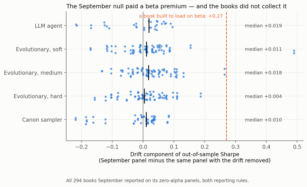
Every book September reported, on the published panel and on its drift-free twin

So September’s headline — that a research agent manufactures an in-sample Sharpe of 2.1 from nothing, and that 88% of it is explained by two integers in the log — stands. The generator does not. It has been replaced, the arithmetic is in the repository, and the correction is in this post rather than in a footnote, because a null you cannot verify is what this entire post is about.

Setup

The null. Factor-structured daily panels: 400 names, regime-switching volatility on the market and three latent factors, Student-t idiosyncratic shocks, lognormal dispersion in volatility. Zero drift, symmetric clipping, and — the part the September generator got wrong — separate random streams for structure (betas, loadings, volatilities, regime paths) and for innovations, so a fresh path can be drawn through the same world.

Verifying that a null is null is harder than writing one. The pre-registered acceptance test probed a constant-beta book and two oracle signals; it passed on two and, on the third, produced a +0.093 on the sixty study seeds that went away on a 120-seed replication. That episode is in the deviations file, and the acceptance file records the pre-registered failure rather than only the replication that passed. It also convinced me the test was too blunt, so there is a better one: 200 expressions drawn from the signal grammar before any panel existed, of which a median of 184 evaluate cleanly on a given panel, across 40 fresh null panels — 7,346 signal-panels, mean annualised Sharpe +0.017, 95% CI [−0.015, +0.048].

Two honest caveats on that. It is measured on the 1,000-day training window, not on the 2,000-day window the books are scored on. And on the exact sixty seeds this study ran, the residual tilt from the acceptance test is bounded at about +0.09 — larger than several of the out-of-sample numbers below. I flag them where they appear.

The pipeline being controlled. An evolutionary search over the same price-only grammar as the September post — returns, moving averages, rolling moments, range position, rolling beta and correlation, with cross-sectional and time-series normalisations. Twelve rounds of twenty-five expressions. The uncontrolled baseline reports the three highest in-sample Sharpes as an equal-weight book. Sixty seeds (9000–9059); 1,000 training days; 2,000 untouched days for scoring.

The two things worth measuring. Every control is placed on two axes.

How much manufactured Sharpe does it remove? Measured on panels with no alpha, and — this matters more than it sounds — measured on the number a user of that control would actually report. If a gate abstains, nothing is reported. If a control re-selects on a validation window, the researcher reports the validation-window number, not the training number they just threw away. If a control searches a shorter window, the researcher reports the shorter window’s Sharpe. Measuring every control on the original training window, which is what I did in the first pass of this study, flatters every re-selection control enormously and is the single largest correction here.

How much real alpha does it destroy? Measured on the same panels with a signal planted in them. Because each seed’s panels are drawn from identical innovations and differ only in the plant, the same book can be scored on both, which separates the exposure a noise-selected book has to the plant by construction from the gain that selecting on the planted panel actually adds. Only the second is “finding alpha”.

Two plants, and why. My first plant was calibrated to an in-sample Sharpe of about 1.0 — below the 1.77 the search manufactures from noise. A pipeline that ranks on in-sample Sharpe must then prefer the noise, so “the search fails to find real alpha” was a property of my calibration rather than a finding. There are now two, both calibrated on thirty seeds (8000–8029) rather than the three the first pass used: a weak plant and a strong one, with realised out-of-sample oracle Sharpes on the study seeds of 0.59 and 2.43.

The analysis plan, the predictions and the estimators were committed before the first search ran. Eighteen departures from them are logged, including several this study’s reviewers forced.

1. Selection manufactures the Sharpe. The search adds nothing.

Start with the uncontrolled pipeline on panels containing nothing:

Uncontrolled pipeline, 60 null panelsValue
Reported in-sample Sharpe1.77 (SE 0.04)
Realised out-of-sample Sharpe, 2,000 days+0.015 (SE 0.051)
One-way turnover, per day19.5%
Net of 5 bp per unit of turnover, at ≈2.5% book volatility−1.00

Familiar enough. Now the part I did not expect. Take 200 expressions drawn at random from the grammar before any panel is generated — no search, no feedback, no breeding — and keep the best three by in-sample Sharpe. On the same kind of null panel that book has an annualised in-sample Sharpe of 1.99 (SE 0.05, 40 panels).

Put the evolutionary search on exactly the same footing — its own logged candidates, the same 700-day window, the same complete-case filter, top three re-selected on that window — and it reports 1.95 (SE 0.05, 60 panels). The difference is 0.04, Welch t = 0.60.

Twelve rounds of adaptive search, three hundred evaluations, mutation and crossover, and the machinery adds nothing measurable to the manufactured number. Picking three things out of a hundred and eighty-odd does all of the work. (The two arms run on different seed sets and are not paired; the pools are matched at 182 against 184 candidates after filtering, with participation ratios of 13 and 15.)

Whatever your research process is — an agent, a grid, a graduate student with a notebook — the quantity that produces the fictitious Sharpe is the size of the set you chose from, and nothing clever has to have happened inside.

2. The holdout that made the number bigger

Here is the reported in-sample Sharpe on panels with no alpha, for each control, measured on the window that control actually reports:

ControlReported Sharpe, null panelsManufactured Sharpe removedAbstains
Internal gate (search 750 days, pick on 250)3.08−0.74—
Internal gate + leg cap of 12.45−0.38—
750-day search, no gate2.15−0.22—
Leg cap 121.78−0.01—
Uncontrolled baseline1.77——
Leg cap 11.650.07—
Budget 6 × 251.590.10—
Budget 12 × 121.560.12—
Budget 6 × 121.420.20—
Out-of-path gate (fresh innovations)1.360.23—
CSCV / PBO gate1.080.3925 of 60
Romano–Wolf stepdown0.410.7748 of 60
Deflated Sharpe hurdle0.001.0060 of 60

Read the last column before the middle one. For the three gates, the removal figure is driven by the abstention rate rather than by any reduction: those gates never make a fiction smaller. They make it rarer — and on the panels where Romano–Wolf does pass, the book it lets through reports 2.04, above the 1.77 it was meant to discipline; the PBO gate’s pass-conditional number is 1.85. That is why each gate’s removal figure sits below its abstention rate — 0.77 against 48 abstentions in 60, 0.39 against 25 — and it means that conditional on getting an answer out of them, you get a worse number than if you had not asked.

Now the top of the table. The train/validate split is the most widely practised control in quantitative research, and on a panel with no alpha it made the reported number 74% larger.

The mechanism is not subtle once you see it. On a panel with no alpha, every point of reported Sharpe is selection. The standard error of a Sharpe estimate scales as one over the square root of the sample, and for a fixed candidate pool the expected maximum scales with that standard error — so the ratio of two reported maxima should be the square root of the inverse ratio of their sample sizes. Those sample sizes are the days the Sharpe is actually computed over, after each book’s warm-up is dropped: 876 for the baseline, 591 for the 750-day search, and a clean 250 for the validation window, which needs no warm-up.

Predicted: √(876/591) = 1.2172 and √(876/250) = 1.872. Observed: 1.2175 and 1.742. The first is right to three decimal places. The gate falls a little short of its prediction because it selects from a pool bred on a different window, so its candidates are not the baseline’s candidates.

Look at the “750-day search, no gate” row, which is there precisely to separate the two effects. Running the same shorter search and reporting its own window’s top three already inflates the number by 22%. The gate adds a further 52 points of the baseline on top of that. Splitting the sample does not remove the selection: it relocates the selection to a shorter window, where selection is cheaper and its rewards are larger — and then hands you that number to report. This is the practical form of a result that is already well established in adaptive data analysis: a holdout reused for selection stops being a holdout [8].

The same logic hits the out-of-path gate, which I expected to be the best control in the study. It re-scores every candidate on a genuinely fresh path through the same world and keeps the best three. A top-three-of-two-hundred maximum over 1,000 fresh days is still worth 1.36. The gate does not remove the manufactured Sharpe. It moves it onto a new path and lets you report it there with a clear conscience.

If a control ends by selecting a maximum, the maximum is the problem, and the control has not addressed it.

One anticipation. A 750/250 split is not a straw split — 70/30 and 80/20 are the conventional choices, and the effect gets worse as the validation window shrinks, so a shop splitting 80/20 on four years is further along this curve than the one measured here.

3. The corrections are fine. You are pointing them at the wrong family.

Three of these controls are formal multiple-testing procedures with published guarantees: the deflated Sharpe ratio [1], the CSCV probability of backtest overfitting [2], and a Romano–Wolf stepdown at 5% familywise error [3], bootstrapped with a stationary block bootstrap [4]. Their realised size on null data is well known to be disappointing in practice. The question that seems not to get asked is whether that is the procedure’s fault.

So I measured each twice: once on the family of candidates the search produced, and once on a family of 200 expressions fixed before the data existed.
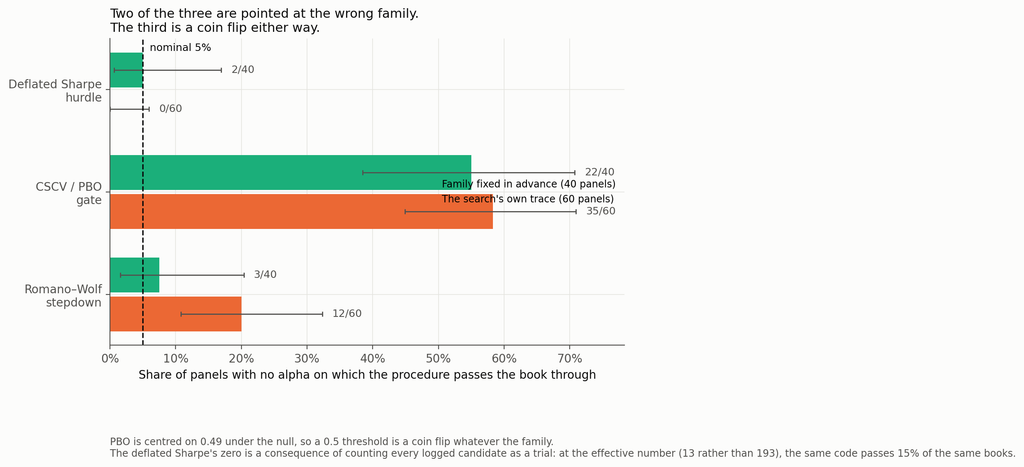
Realised size on a family fixed in advance against the search’s own trace

ProcedureFamily fixed in advance (40 panels)The search’s own trace (60 panels)
Deflated Sharpe hurdle2 of 40 (5%)0 of 60 at N = 193 logged; 9 of 60 (15%) at N effective = 13
CSCV / PBO gate22 of 40 (55%)35 of 60 (58%)
Romano–Wolf stepdown3 of 40 (8%)12 of 60 (20%)

On a family chosen before the data I can detect no inflation in either formal procedure. Forty panels is not enough to certify a 5% test — the Romano–Wolf interval runs from 1.6% to 20.4% — so read that column as the absence of the gross inflation the search family produces, not as a calibration certificate. What is unambiguous is the other side. Pointed at the family the search produced, Romano–Wolf rejects on 12 of 60 panels containing nothing: four times nominal, binomial p < 10⁻⁴. Forty panels against sixty is too little to make the 8%-versus-20% contrast itself significant — Fisher’s exact test on that comparison gives p = 0.15 — so the claim that carries is the one against nominal, not the one across columns. The size inflation on the search family is also not a bootstrap artefact: it holds at expected block lengths of 5, 21 and 63 days and at 500 and 2,000 replications, ranging from 18% to 20% across all four settings.

Why? Not because the bootstrap fails to see the generations that bred the survivors — restrict the family to the search’s round-zero population, random expressions no selection has touched, and rejections fall from 12 panels to 6 (paired exact p = 0.07). That points at adaptive breeding as one contributor rather than the whole story; on sixty panels it is a direction, not a decomposition. The rest is the plainer fact that the family was chosen by looking at the window the test then uses.

The deflated Sharpe ratio is a more uncomfortable case, because its answer is determined by a number you supply. It needs the number of trials; I gave it the count of distinct expressions the search logged, a mean of 193 across panels (range 103 to 258). Those are not independent trials — the participation ratio of their correlation matrix averages 13 (range 5 to 26). Feeding 193 independent trials into a formula that assumes independence pushes the expected-maximum benchmark above the book’s Sharpe on 40 of 60 panels, and leaves the z-statistic short of the 95th percentile on the other twenty — so the hurdle rejects everything. Feed it 13 and the same code, on the same books, passes 9 of 60 — three times nominal (p = 0.003), in the opposite direction. The control’s verdict is a function of a modelling choice nobody documents. To be clear, no published implementation asks for an effective trial count; this is an extension of the method, not a correction to it.

And then there is PBO, which I had been treating as a control and which is not one. CSCV’s logit statistic is symmetric about zero when the candidate strategies are exchangeable and null, so the probability of backtest overfitting is centred on 0.49 — by construction, not by accident. A threshold at 0.5 is therefore a coin flip on data containing nothing: it passes 55% of pre-specified null books and 58% of searched null books. It is not powerless — against the strong plant it passes 95% — but a gate whose false-pass rate is 58% is not a 5% test, whatever it does on real signal.

4. What the controls cost you

Removing fiction is half of a control’s job. The other half is not destroying the thing you are looking for, and you cannot measure that on a null panel.

Against the strong plant — realised out-of-sample oracle Sharpe 2.43, above what the search can manufacture — here is what each control finds of it, alongside what it removes:
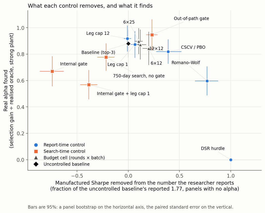
What each control removes and what it keeps

The right-hand column is the selection gain defined in the Setup — what selecting on the planted panel adds over what a null-selected book earns on it by construction. The raw ratio of book Sharpe to oracle is lower, because a book’s exposure to the plant is slightly negative on average: 0.81 for the baseline and 0.85 for the out-of-path gate.

ControlManufactured Sharpe removedReal alpha found (selection gain ÷ oracle)
Out-of-path gate0.230.95
Leg cap 12−0.010.92
Budget 6 × 250.100.90
Uncontrolled baseline—0.88
Leg cap 10.070.87
Budget 12 × 120.120.87
Budget 6 × 120.200.84
CSCV / PBO gate0.390.82
750-day search, no gate−0.220.78
Internal gate−0.740.67
Romano–Wolf stepdown0.770.60
Internal gate + leg cap 1−0.380.57
Deflated Sharpe hurdle1.000.00

The minimum difference detectable at 80% power between the baseline and any of the seven pre-registered controls in that column, after Holm across the whole 84-test scan, runs from 0.05 to 0.21 of the oracle. Differences smaller than that should not be read — including the gap between the out-of-path gate’s 0.95 and the uncontrolled baseline’s 0.88, which is nominally the largest in the table and is not separable at this sample size.

The deflated Sharpe hurdle rejects a genuine 2.4-Sharpe strategy on all sixty panels, and passes exactly one of the sixty carrying the weak plant. Its perfect score in the removal column and its zero in the retention column are the same fact stated twice. A control that abstains on everything is unfalsifiable on null data and useless on real data, and you cannot tell those two properties apart without running a planted arm.

Romano–Wolf is the most defensible trade in the table: it removes 77% of the fiction — by abstaining four times in five — and keeps 60% of a strong real signal. That is a real control with a real price, which is more than most of this column can claim.

The out-of-path gate keeps the most alpha while removing a real 23% of the fiction. It is the only control whose null-panel out-of-sample Sharpe is even marginally negative (−0.086, SE 0.045, 95% CI [−0.17, +0.00]) — a t of 1.9 in a scan across fourteen arms, and inside the residual-tilt bound I flagged in the Setup, so I would not lean on the sign.

Four controls dominate the internal gate on both axes after Holm adjustment: leg cap 1, leg cap 12, the out-of-path gate, and — awkwardly — the PBO gate I have just described as a coin flip. No other pair dominates. That a gate with no size control still dominates the internal gate says more about the internal gate than it does about PBO.

A fourteenth arm, the shorter search with a leg cap of 1, is in the repository and not in these tables: it reports 2.01 on null panels — a little less inflation than the window-matched arm’s 2.15 — and finds 0.78 of the plant, which is the window-matched arm’s figure to within noise.
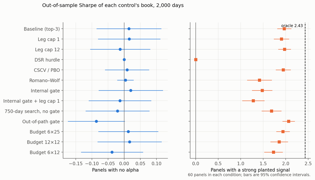
Out-of-sample Sharpe of each control’s book, with no alpha and with a strong plant

One more thing this table only shows because there is a strong plant in the study. Against the weak plant — oracle 0.59 — the uncontrolled pipeline’s selection gain is 11% of the oracle with a minimum detectable effect of 27%. That is not a finding, it is a non-detection, and the first pass of this study reported it as “the search captures 6% of the real signal”. The honest version is conditional and worth stating precisely: a search that ranks on in-sample Sharpe finds real alpha when the real alpha is larger than the alpha it can manufacture, and there is no evidence either way when it is smaller.

5. The agent behaves much like the machine

Eighteen fresh runs of the September research agent through a gated harness, six per condition, with the prompt frozen:

ConditionReported in-sampleRealised out-of-sampleOracleFound the plant
No alpha1.41−0.16 (SE 0.12)——
Weak plant1.52+0.24 (SE 0.17)0.503 of 6 exactly, 4 of 6 by family
Strong plant2.91+2.04 (SE 0.16)2.313 of 6 exactly, 6 of 6 by family

Manufactures on nothing, indistinguishable from noise against a weak signal, and its book earns 88% of the strong plant’s oracle out of sample against the mechanical pipeline’s 81% on the same raw basis. The arms ran on different panels and are not formally compared; qualitatively, whatever an LLM researcher is doing, it is not different enough from an evolutionary search to warrant a different control regime.

The arm is not blinded: the run id the agent types on every harness call carries the condition, K0, K1 or K2. Nothing in the logs refers to it, but it was in front of the agent, and six runs per condition is a small arm.

Two details worth having. The agents worked harder when there was more to find — 4.2 evaluation batches of a permitted 12 against the weak plant, 8.5 against the strong one — but they did not stop early on the null panel, where they used 5.7 batches and one run burned all twelve. That is responsiveness to signal strength, not an ability to notice there is nothing there.

And the twelve September agent traces, re-scored under the report-time controls on drift-free panels, behave as the mechanical arms do: the deflated Sharpe hurdle passes 0 of 12, PBO 5 of 12, Romano–Wolf 7 of 12. The exception is leg caps, which move an agent’s reported Sharpe by +0.02 on average at a cap of one and −0.02 at a cap of twelve — never by more than 0.29 on any single run, and in no consistent direction — because an agent’s legs live inside a single expression rather than in the count of expressions. Any control that counts expressions is close to blind to an agent.

6. One real path, for illustration

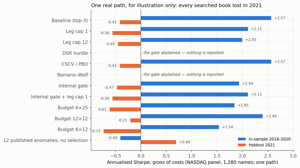
The same pipeline on a real panel — 1,280 NASDAQ names, search 2018–2020, holdout 2021 [5]. One path, a stale and survivorship-conditioned dataset, and a universe filter that looks at the whole sample. It evidences nothing; it is here because it makes the synthetic result legible.

BookIn-sample 2018–2020Holdout 2021Through May 2023
Baseline (top-3)+2.57−0.41−0.24
Leg cap 1+2.11−0.56−0.45
Leg cap 12+2.00−0.45−0.26
CSCV / PBO (passed)+2.57−0.41−0.24
Internal gate+1.94−0.47−0.26
Internal gate + leg cap 1+2.11−0.56−0.45
Budget 6 × 25+1.85−0.61−0.52
Budget 12 × 12+2.40−0.21−0.30
Budget 6 × 12+1.54−0.73−0.64
Deflated Sharpe hurdleabstained——
Romano–Wolfabstained——
Twelve published anomalies, no selection−0.40+0.69+0.69

Every searched book on the real panel, in sample and out

Every searched book turned negative. The unselected canon, which looked worst in sample, was the only thing that worked out of sample. Consistent with the synthetic result, and worth precisely as much as one path is worth.

One inconsistency to flag rather than let a reader find: the in-sample column here is the full 2018–2020 window for every book, including the internal gate, so it is not the reported-window number section 2 corrects to. On this arm the gate therefore appears to lower the in-sample figure when the synthetic result says it raises the number the gate’s user would report. The real panel’s dataset is fetched over the network and I could not re-score that row from the sandbox this study ran in; it is stated here rather than quietly left in the table.

The pre-registration scorecard

PredictionVerdict
P1 the out-of-path gate dominates the DSR hurdle on both axesRefuted, with each control winning one axis: the out-of-path gate removes 1.36 less of the reported Sharpe (CI [−1.45, −1.27]) and finds 2.07 more of the plant (CI [+1.92, +2.21])
P2 a leg cap of 1 removes ≥ 0.20 more than the smallest budget cellRefuted: −0.13, CI [−0.19, −0.07]
P3 the DSR hurdle’s size exceeds 25%Refuted: 0 of 60, conditional on N = logged candidates
P4a the internal gate costs ≥ 0.10 Sharpe on planted panelsConfirmed: −0.49, CI [−0.69, −0.29]
P4b the internal gate removes ≥ 0.50 of the manufactured SharpeRefuted, and in the opposite direction: −0.74

Things that did not work

The leg axis. Capping a book at one leg removes 0.13 less manufactured Sharpe than the smallest search budget does — the budget axis beat the leg axis, and leg caps are close to a no-op on this pipeline. Against an agent they are a complete no-op, for the reason in section 5. This is the one place where I expected a result from the literature to transfer and it didn’t: in-sample statistics do inflate with the number of combined signals [9], but not in a way a cap on the count can reach when the signals are themselves sums.

The pre-registered “oracle frontier” — thresholding candidates on their true out-of-sample Sharpe to trace the best attainable trade-off — is not reported at all. Estimating “true” out-of-sample Sharpe on the same window that scores the books is circular, and on null panels it obligingly produced a frontier that “retained” +0.60 of Sharpe that does not exist. The file is in the repository; the chart does not draw it.

And the first version of this study, which four reviewers took apart before publication. The largest correction was measuring each control on the number a researcher reports rather than the number they discard, which reversed the sign of the headline. The second was noticing that my planted signal had been calibrated to a level the search could beat by fabrication, which made one of my conclusions a property of the experiment rather than of the world. The third was catching three numbers quoted from the weak-plant arm where the text said otherwise. The fourth was showing that this post’s own draft compared the random family and the search on different windows, which inflated the gap in section 1 into a result it is not. All eighteen deviations are logged, and the first-pass tables sit in the repository beside the corrected ones.

What this does and does not show

It does show that on a verified-null panel an in-sample Sharpe of about 1.9 comes out of selecting three candidates from a couple of hundred, on the window the selection is made, and that twelve rounds of adaptive search add nothing measurable to that number.

It does show that a held-out validation window, used the way it is normally used, raises the reported Sharpe rather than lowering it, by roughly the factor the standard error of a Sharpe estimate predicts; and that a fresh-path re-test mostly relocates the manufactured Sharpe rather than removing it.

It does show that two of the three formal procedures show no detectable inflation on a family fixed in advance and are grossly mis-sized on a family the search selected; and that the third is centred on its own threshold under the null and therefore does not decide anything about size.

It does show that a pipeline, mechanical or agentic, recovers most of a planted signal strong enough to beat what it can manufacture — and that the deflated Sharpe hurdle, as conventionally parameterised, destroys all of it.

It does not show that any of these procedures is wrong. Each is implemented here against its published definition and is doing what it was designed to do on the input it is handed.

It does not show anything about faint alpha. Against a signal with a 0.59 oracle Sharpe this design cannot separate “finds nothing” from “finds a quarter of it”. That needs more panels or a longer scoring window.

It does not show a ranking of controls that transfers. The removal axis depends on the reporting convention, the retention axis on a plant that happens to be a single expression the grammar can write exactly — evaluated verbatim by the mechanical search on only 6 of the 60 strong-plant panels, so its findability is not an artefact of expressibility, but a plant the grammar cannot write at all would give a different answer. The leg-cap results depend on a grammar in which a leg is a separate expression, and every net-of-cost number on a book volatility of about 2.5%.

It does not show anything about real markets. One path on a stale dataset is an illustration.

So what do you do?

Report the number you selected on, and say which window it is. Most of the apparent power of every re-selection control in this study came from measuring it on a window the researcher had already discarded: the out-of-path gate’s removal falls from 0.99 to 0.23 when you do this properly, and the internal gate’s flips sign, from +0.47 to −0.74. If your validation split produces a Sharpe of 3.1 where your in-sample fit produced 1.8, the honest headline is 3.1, and the fact that it is larger should alarm you rather than reassure you.

Write down the family before you look. Not the trial count — the family. Every procedure in section 3 shows no inflation on a family fixed in advance and gross inflation on a family your search selected, and the difference between those is a decision you make before the data, not a correction you apply after it.

If you use the deflated Sharpe ratio, state how you counted trials, and report the effective number alongside the raw count. The gap between 193 and 13 on the same candidate set moved the pass rate from 0% to 15%. No published implementation asks for an effective count, so this is an extension rather than a fix — but a DSR quoted without saying how trials were counted is a number with a free parameter in it.

Stop using a PBO threshold of 0.5 as a gate. It is centred on 0.49 under the null. Use the distribution, or use something else.

Run a planted arm. This is the one that costs real effort and is worth it. A control that abstains on everything looks perfect on a null panel; you only find out what it costs when you give it something real to find. And calibrate the plant above what your own pipeline can fabricate, or you will measure your calibration rather than your control — which is exactly what the first version of this study did.

Code and data

The repository holds the pre-registered analysis plan committed before the first run, eighteen logged deviations from it, the corrected generator with its bitwise verification against the September panels, the calibration of both plants, the full study across 180 panels, the pre-specified-family placebo, the erratum arithmetic against all 294 previously published books, the agent harness with every run log and journal, the canary tests, and the analysis and figure code. Seeds: study panels 9000–9059, calibration 8000–8029, placebo panels 9500–9539, pre-specified family drawn from seed 20260921. Everything except the LLM calls reproduces from those seeds; the LLM calls are not re-runnable, which is why the logs are included in full. The repository is at github.com/jkinlay/research-controls; this article refers to commit c11241e.

Two requests of anyone re-running it. Fix your family before you look at the data, and keep the list. And run a planted arm alongside the null arm — half the results here are invisible without one.

References

[1] Bailey & López de Prado, The Deflated Sharpe Ratio: Correcting for Selection Bias, Backtest Overfitting and Non-Normality, Journal of Portfolio Management 40(5), 2014.

[2] Bailey, Borwein, López de Prado & Zhu, The Probability of Backtest Overfitting, Journal of Computational Finance 20(4), 2017; and Pseudo-Mathematics and Financial Charlatanism, Notices of the AMS 61(5), 2014, for the expected-maximum-Sharpe result.

[3] Romano & Wolf, Stepwise Multiple Testing as Formalized Data Snooping, Econometrica 73(4), 2005, 1237–1282. The stepdown implemented here is the one-sided studentised version at 5% familywise error.

[4] Politis & Romano, The Stationary Bootstrap, Journal of the American Statistical Association 89(428), 1994. Expected block length 21 days throughout. The section 3 size result is stable across that choice: 18% at a block length of 5, 20% at 21, 18% at 63, and 18% at 21 with 2,000 replications rather than 500.

[5] skfolio, load_nasdaq_dataset — daily adjusted closes, 1,455 NASDAQ constituents, 2018-01-02 to 2023-05-31, documented by its authors as a stale dataset not intended for investment or commercial use. Filtered here to 1,280 names with median price ≥ $5.

[6] Harvey & Liu, Backtesting, Journal of Portfolio Management 42(1), 2015 — the multiple-testing haircut the report-time controls in section 3 descend from.

[7] Harvey & Liu, False (and Missed) Discoveries in Financial Economics, Journal of Finance 75(5), 2020, on the two-sided cost of correction; section 4 is a direct measurement of the missed-discovery side. See also Chen, The Limits of p-Hacking: Some Thought Experiments, Journal of Finance 76(5), 2021, 2447–2480, for the argument that selection alone cannot account for the observed cross-section — the complement of the measurement in section 1.

[8] Dwork, Feldman, Hardt, Pitassi, Reingold & Roth, The reusable holdout: Preserving validity in adaptive data analysis, Science 349(6248), 2015. Section 2 is the practical, one-reuse form of the result that a holdout used for selection stops being a holdout.

[9] Novy-Marx, Backtesting Strategies Based on Multiple Signals, NBER Working Paper 21329, 2015, on the inflation of in-sample statistics with the number of combined signals — the leg axis that section 4 finds to be a no-op here.

Disclosure: I run systematic strategies. Nothing here is a recommendation, and no strategy discussed is one I trade. These are diagnostic quantities from a methodological experiment on synthetic data and one stale public dataset, not a track record.

Deep Learning for Volatility Surface Repair

A self-contained synthetic benchmark of a small mask-conditional CNN against calendar-projected linear interpolation and a per-slice SVI fit.

A volatility surface marker is rarely a clean rectangle of quotes. Strikes go unobserved during illiquid hours, wings get crossed and then erased, broker stripes drop out across an entire maturity, and weeklies arrive at the desk with random missingness on top of base quote noise. Anyone calibrating an SVI surface or running an SSVI fit operationally is doing it on top of an upstream repair step, whether that step is explicit or not. The repair step is usually some flavour of local interpolation, sometimes followed by a no-arbitrage projection, sometimes pre-empted by a model-based smoother.

The question I want to put a number on is whether a small learned model can compete with the local approach in this repair role. The reason to ask is that a learned model, in principle, knows something about the joint structure of plausible volatility surfaces that a local interpolator does not — vol surfaces are not arbitrary functions on a (k, T) grid, they have term-structure shape, characteristic skew patterns, ATM smoothness — and a model that has seen a thousand surfaces should be able to use that prior to improve on local interpolation, especially where local data is thin.

The reason to be sceptical is that local methods are very strong at what they do. Linear interpolation in (T, k) is unbiased, has no parameters to overfit, costs nothing operationally, and is hard to beat on smooth surfaces with reasonable observation density. Per-slice SVI gets you smile shape correctly even when only a handful of strikes are observed, provided the slice has enough quotes to fit. Beating both of those baselines requires that the learned prior contributes something local methods cannot — and the most plausible places for that to happen are when local data is too sparse for SVI to fit and too irregular for interpolation to fill the gap cleanly.

This note runs that experiment on synthetic data. It is deliberately a small CNN rather than a U-Net or a VAE, partly because that is the smallest interesting architecture for this problem, and partly because if a small model cannot establish a foothold here, the question of whether to build something larger has a clearer answer than if it can.

The full code is in vol_surface_repair.py; it runs on CPU in roughly four minutes.

Setup

Grid. Maturities and log-moneyness on a 13 × 17 grid: T \in [0.08, 2.0] (years), k \in [-0.45, 0.45]. All surfaces are stored as total variance w(k, T) = \sigma^2(k, T)\, T; evaluation metrics are computed in implied-vol units (\sigma) for interpretability.

Training surfaces. 1600 SSVI surfaces drawn from a fairly tight parameter range:

theta0 = U(0.010, 0.032)        # ATM total variance at front
theta_slope = U(0.020, 0.070)   # linear term in maturity
theta_curve = U(-0.006, 0.010)  # quadratic term
rho = U(-0.72, -0.18)           # skew
eta = U(0.55, 1.55)             # SSVI eta
gamma = U(0.18, 0.62)           # SSVI gamma

Calendar monotonicity is enforced on the clean target via cumulative maximum along T so the model is never rewarded for learning calendar arbitrage from the simulator. A 200-surface validation set, drawn from the same parameter range with different seeds, is held out for best-checkpoint selection.

Test surfaces. Two test families, each with 200 surfaces per cell and seeds independent of training:

  • Shifted SSVI — same generator with widened parameter ranges and an occasional maturity-localised bump. The generator is in-distribution in form but stress-tests the boundaries.
  • SABR-style event — a separate generator deliberately not identical to SSVI, with square-root maturity decay in ATM vol, stochastic skew term-structure, asymmetric wings, and occasional event-maturity bumps and kinks. This is the out-of-distribution test: smile structure that the model has never seen.

Both families are then perturbed by realistic quote noise (~18 bps in vol space, with wing- and front-end inflation) and masked according to one of two missingness regimes:

  • Regular — about 50% observation density, modest wing deletions, occasional broker-style stripes.
  • Adversarial — about 18% observation density, large contiguous wing or maturity holes, with a thin ATM spine and a few scattered anchors restored so the problem remains solvable but is genuinely sparse.

The result is a 2 × 2 evaluation: {shifted SSVI, SABR-event} × {regular, adversarial}. The motivation is to disentangle two different ways the repair task can be hard: hard because the model has not seen this surface family before, and hard because the available data is too sparse for any local method to cope.

Baselines. Two of them.

  • Calendar-projected linear interpolation: triangulated linear interpolation in (T, k) on observed total variance, with a nearest-neighbour fallback for points outside the convex hull, followed by a cumulative-maximum projection along T to enforce calendar monotonicity. Unparameterised, fast, hard to beat on smooth surfaces.
  • Per-slice SVI fit: at each maturity, a coarse raw-SVI grid search over (\rho, m, \sigma) with the best (a, b) solved in closed form by least squares. Faster than nonlinear least squares, adequate as a baseline. Followed by the same calendar projection as interpolation. This is the published-textbook approach to surface repair when you have enough quotes per slice.

Both baselines are evaluated on the same noisy/masked inputs as the CNN.

Model

The repair network is a four-layer 32-channel convolutional network with two output heads — a softplus mean head and a clipped log-variance head:

class RepairCNN(nn.Module):
   def __init__(self, in_channels=4, width=32):
       super().__init__()
       self.backbone = nn.Sequential(
           nn.Conv2d(in_channels, width, 3, padding=1), nn.SiLU(),
           nn.Conv2d(width, width, 3, padding=1), nn.SiLU(),
           nn.Conv2d(width, width, 3, padding=1), nn.SiLU(),
           nn.Conv2d(width, width, 3, padding=1), nn.SiLU(),
      )
       self.mean_head = nn.Conv2d(width, 1, 1)
       self.logvar_head = nn.Conv2d(width, 1, 1)
​
   def forward(self, x):
       z = self.backbone(x)
       mean = F.softplus(self.mean_head(z)) + 1e-5  # w / W_SCALE
       log_var = torch.clamp(self.logvar_head(z), -8.0, 1.5)
       return mean, log_var

The four input channels are the masked observed total variance (normalised by W_SCALE = 0.08), the binary observation mask, and two normalised coordinate channels for maturity and log-moneyness. The mean head outputs normalised total variance; the log-variance head produces a heteroscedastic uncertainty estimate.

The output space is total variance rather than implied vol. Both choices are defensible — a controlled experiment with the same training pipeline run in vol space gives essentially identical missing-point RMSE — and total variance has the practical advantage that calendar-arbitrage and butterfly-arbitrage diagnostics are natural in this space.

The loss is a weighted reconstruction term in the normalised w-space, plus a heteroscedastic Gaussian NLL (turned on after a 10-epoch warmup), plus a calendar-arbitrage penalty (penalising negative differences along T in real-w space), plus a small smoothness regulariser:

def repair_loss(mean_norm, log_var, target_norm, mask, cfg, use_nll):
   weights = 1.0 + (cfg.missing_weight - 1.0) * (1.0 - mask)
   sq = (mean_norm - target_norm)**2
   mse = torch.mean(weights * sq)
   loss = mse
   if use_nll and cfg.nll_weight:
       inv_var = torch.exp(-log_var)
       nll = 0.5 * torch.mean(weights * (sq * inv_var + log_var))
       loss = loss + cfg.nll_weight * nll
   if cfg.calendar_weight:
       loss = loss + cfg.calendar_weight * calendar_penalty_w(mean_norm)
   if cfg.smoothness_weight:
       loss = loss + cfg.smoothness_weight * smoothness_penalty(mean_norm)
   return loss

The missing-cell weight is 5x the observed-cell weight, so the model is explicitly graded on its repair quality rather than its ability to denoise observed quotes. The calendar weight is set to 80, which is high enough to drive raw calendar-violation rates into single digits at evaluation time but not so high that it dominates the reconstruction loss during training. The smoothness term is small (0.05 weight) and exists mainly to discourage high-frequency artefacts at the wings.

Training runs for 60 epochs in a single process with AdamW (lr 1e-3, wd 1e-4) and a cosine annealing schedule. The first 10 epochs run pure MSE; the NLL term turns on afterwards to give the variance head an MSE-stabilised mean to train against. A 200-surface validation set is used for best-checkpoint selection by missing-point RMSE in vol units. Batch size 128, gradient clipping at norm 1.0.

I will say a word about training duration because the result is more sensitive to it than I would like. With only 8 training epochs, the model’s missing-point RMSE on shifted SSVI / regular missing is 0.049 in vol units; at 60 epochs it is 0.018. The convergence is slow and the validation curve is still improving slightly at epoch 60. Sixty epochs is therefore a deliberate choice rather than a generous one — at that point the validation curve has flattened enough that further training mostly trades off in-distribution refinement against out-of-distribution generalisation, with no clear winner.

The 2 × 2 result

Headline numbers: missing-point RMSE in implied-vol units, mean ± standard error across 200 test surfaces per cell. Bold marks the best estimator per row, with ties (within one SE) bolded together.

CaseObs %CNNInterpSVI
Shifted SSVI / regular50.5%0.0184 ± 0.00100.0131 ± 0.00080.0191 ± 0.0048
Shifted SSVI / adversarial18.1%0.0527 ± 0.00240.0506 ± 0.00260.0540 ± 0.0123
SABR-event / regular50.4%0.0671 ± 0.00130.0248 ± 0.00110.0189 ± 0.0021
SABR-event / adversarial17.7%0.0960 ± 0.00110.0679 ± 0.00190.0784 ± 0.0089

Four cells, four different stories.

Shifted SSVI / regular. Calendar-projected linear interpolation wins outright: 0.013 versus the CNN’s 0.018. The surfaces here are smooth, the parameter shifts from the training distribution are modest, and roughly half the grid is observed. There is little for a learned prior to add: the local data is dense enough that triangulated interpolation captures essentially all the recoverable structure. The CNN is 40% worse, well outside one SE.

Shifted SSVI / adversarial. The CNN and interpolation are statistically tied (0.053 vs 0.051, within one SE of each other). With observation density at 18% and large contiguous holes, neither method has a clean run, but the CNN’s learned prior on smile shape brings it back into the same neighbourhood as interpolation. The SVI fit is also competitive here, although noisier across surfaces because individual maturity slices sometimes have too few quotes to fit reliably.

SABR-event / regular. SVI wins narrowly (0.019 vs interpolation’s 0.025), the CNN comes in third at 0.067. This is the cell that distinguishes baselines: SVI fits the local smile structure correctly slice-by-slice and pays no penalty for the SABR family being out-of-distribution because it is a per-slice model with no cross-slice prior to mislead it. The CNN, trained only on SSVI surfaces, has learned a prior that does not transfer cleanly to the asymmetric-wings, event-kink SABR family. It is 2.5× worse than SVI here.

SABR-event / adversarial. Interpolation wins (0.068 vs the CNN’s 0.096), with SVI in the middle at 0.078 and noisy because slice-level data is too sparse to fit consistently. The dominant error source for the CNN here is generalisation, not data scarcity. Even with adversarial missingness — exactly the case where one might hope a learned prior contributes most — the OOD penalty dominates.

The pattern across cells is consistent. The CNN is competitive only where its learned prior matches the test distribution and local methods are operating at their weakest. It loses materially when either of those conditions fails. Calendar-projected linear interpolation is the most consistent baseline of the three: it is the best estimator in two cells, statistically tied for best in a third, and the second-best in the fourth.

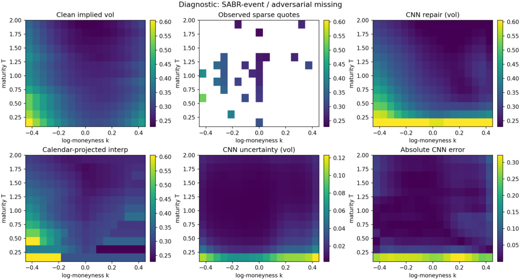
The diagnostic figure below shows a single SABR-event adversarial-missingness example. The observed input has lost a substantial chunk of the wings, the entire long-maturity tail, and the front-maturity strip; what remains is a thin ATM spine and a handful of scattered anchors. The CNN repair is smooth and plausible, with errors concentrated at the front-maturity wings — exactly where the input is most aggressively masked. The uncertainty head correctly flags that region as high-uncertainty. Calendar-projected interpolation produces the characteristic “shelf” artefact at the maturities where the cumulative-max projection has had to adjust the raw output.

Diagnostics

A repair model that minimises missing-point RMSE while producing arbitrageable surfaces and miscalibrated uncertainty is not a usable estimator. The diagnostics below are not the headline; they are the things you have to report in order for the headline to load-bear.

Caseraw cal %post-proj cal %g(k)<0 %cov80cov95err–sd corrstale AUC
SSVI / regular2.650.005.320.690.850.690.66
SSVI / adversarial9.750.007.710.470.630.640.64
SABR / regular2.190.008.730.300.430.760.55
SABR / adversarial11.050.0011.080.280.410.860.55

The honest summary, line by line:

Calendar arbitrage. The raw CNN output violates calendar monotonicity in 2–11% of (k, T) edges across the four cells. The cumulative-maximum projection drives this to zero everywhere. The calendar-projection step is therefore doing real work, and the model should not be deployed without it. The training-time calendar penalty is doing partial work — without it, raw violation rates would be substantially higher — but it is not on its own sufficient to produce calendar-monotone output reliably.

Butterfly arbitrage. Even after calendar projection, 5–11% of grid points exhibit g(k) < 0 under the discrete Gatheral–Roper diagnostic, with the worst rates on the SABR cells where the CNN is least confident. The smoothness penalty in the loss does not buy enough convexity to fix this. A real butterfly-arbitrage projection — one that actually projects onto the no-arbitrage manifold along k rather than just regularising — would be the right next step. I have not done it here, and the post-projection g(k)<0 rate is the most concerning single number in this set of diagnostics.

Uncertainty calibration. The heteroscedastic head undercovers. Nominal 80% intervals deliver 28–69% empirical coverage; nominal 95% intervals deliver 41–85%. The error-versus-predicted-sd correlation is positive everywhere (0.64–0.86), so the model is at least directionally aware of where its output is unreliable, but it is overconfident about how unreliable it is — particularly on the OOD SABR cells, where the variance head has nothing to recalibrate against. This is the standard limit of in-training Gaussian NLL: under distribution shift, the variance head is as miscalibrated as the mean head, in the same direction. A held-out conformal step is the obvious fix and would be the cheapest single change to make the uncertainty channel operationally useful.

Stale-quote AUC. A synthetic test: inject stale errors into 8% of observed quotes, run the model on the stale-injected surface, and compute the AUC of the residual |obs – \mu| as a stale-quote score. Numbers come in at 0.55–0.66. Better than chance, but weak — particularly on the OOD SABR cells where the AUC sits just above 0.55. This says the model’s residual is not, on its own, a strong stale-quote detector. A more useful operational stale-detection pipeline would combine the model residual with quote-time and quote-source signals, and the model is contributing a useful but limited fraction of the discriminative signal.

Downstream SVI projection

Surface repair is a means to an end. What the calibration desk usually wants is a smooth, arbitrage-projected SVI surface, not the raw repair output. A repair that is more accurate in the missing-point RMSE sense but less amenable to clean SVI projection might be a worse operational deliverable than the reverse. The right question is not just “how accurate is the repair” but “how good is the SVI fit to the repaired full surface”.

To get at this, I run a per-slice SVI projection on the full repaired surface (CNN or calendar-projected interpolation), then re-score the SVI fit against the held-out missing cells:

CaseSVI after CNNSVI after interp
Shifted SSVI / regular0.0171 ± 0.00270.0159 ± 0.0071
Shifted SSVI / adversarial0.0401 ± 0.00800.0426 ± 0.0113
SABR-event / regular0.0697 ± 0.00500.0295 ± 0.0062
SABR-event / adversarial0.0913 ± 0.00570.0634 ± 0.0065

The downstream metric does not change the qualitative ranking: CNN-then-SVI narrowly beats interp-then-SVI on the cell where the headline RMSE was already tied (SSVI / adversarial), and loses everywhere else. The CNN is not producing surfaces that are pathologically uncooperative under SVI projection — the SVI residuals follow the missing-point RMSE residuals reasonably faithfully. That is mildly reassuring from a deployment perspective: the choice between estimators is not being secretly arbitraged away by the projection step.

What this experiment shows and does not show

A small mask-conditional CNN, trained on 1600 synthetic SSVI surfaces under explicit calendar and smoothness penalties, with 200 validation surfaces for checkpoint selection, can repair sparse and noisy total-variance surfaces under a tight enough discipline that it:

  • produces calendar-monotone output after a cumulative-maximum post-projection (which both baselines also need);
  • matches calendar-projected linear interpolation, within statistical noise, on adversarial in-distribution missingness;
  • loses to interpolation by roughly 40% on benign in-distribution missingness, where the local-data density is high enough that triangulated interpolation captures essentially all the recoverable structure;
  • loses by a factor of 1.4–2.7× on out-of-distribution SABR-style smiles, depending on observation density;
  • carries a heteroscedastic uncertainty estimate whose direction is right (positive correlation with error) but whose magnitude is undercalibrated, particularly under distribution shift.

What this experiment does not show, and what I want to be plain about:

It does not show that this kind of CNN-based repair is useful on real data. The synthetic surfaces have no calibration drift, no quote-time-of-day noise, no microstructure asymmetries, no realistic smile dynamics, no hard-to-fit weeklies or single-name idiosyncrasies. The repair task here is pristine compared to anything one would do on production market data. Whether the small relative gap between CNN and interpolation on the adversarial cell survives a real-data test is an open question that this experiment cannot answer.

It does not show that a CNN is the right architecture for this task. A four-layer 32-channel CNN on a 13 × 17 grid is the smallest interesting model for this problem; a U-Net, an attention-conditioned masked decoder, or a conditional VAE all have published precedents in the volatility-repair literature and would be plausible candidates for materially better performance. The choice here was deliberate — keep the model small and the comparison clean — but it is not the architecture I would deploy if I were trying to win the headline number.

It does not show that the SABR-event family is the right test for OOD generalisation. The CNN is being asked to handle smiles whose convexity term-structure and wing asymmetry have a different functional form from anything in its training set. That is a hard test by design, and the gap to SVI on SABR / regular says that what the CNN has learned is closer to “the SSVI smile family” than “smile structure in general”. A more useful experiment would mix multiple smile families during training and re-test on a held-out one.

It does not, on its own, justify a production system. Before this estimator went anywhere near a market-making book it would need a real-data study, downstream P&L attribution, a much more serious calibration of the uncertainty head, a butterfly-projection step, and a comparison against more competitive learned baselines.

Where to take this next

Roughly in priority order:

  1. Real-data replication. Run the same 2 × 2 on an index-options panel across a year — in-sample dates against out-of-sample dates, regular trading days against unusually sparse ones — and see whether the conditional pattern survives. This is the single biggest credibility step. Everything in this note is conditional on the synthetic setup being a reasonable proxy for production data, and that conditioning is not free.
  2. No-arbitrage projection. Add a full butterfly-arbitrage projection alongside the calendar cumulative-max, and report whether forcing the CNN onto the no-arbitrage manifold during evaluation changes the ranking. The 5–11% post-projection g(k)<0 rate is the most uncomfortable number in the diagnostics.
  3. Calibrated uncertainty. Replace the in-training heteroscedastic NLL with a conformal wrapper trained on a held-out residual set, or with a deep ensemble across seeds. The current undercoverage on OOD cells is bad enough that the uncertainty channel is more decorative than useful.
  4. Mixture training. Train on a mixture of smile families (SSVI plus SABR-event plus a Heston-like family) and re-test on a held-out family. The SABR loss is dominantly a generalisation failure, and the cheapest single fix is to broaden the training distribution.
  5. Generative baseline. Compare a small VAE on the same harness, conditioned on the missingness pattern, as the published baseline for learned vol-surface repair. The conditional-on-mask deterministic CNN here is probably not the right architecture in the limit.

None of these requires a deep architectural rethink. They are mostly questions of where the experiment runs and what it gets compared against.

Code and references

The full script (vol_surface_repair.py) is self-contained, CPU-friendly, and reproducible: it generates the training and test data, trains the CNN, evaluates against both baselines, computes the diagnostics, runs the downstream SVI projection, and writes the figure and the numeric results to disk. Run with python vol_surface_repair.py. Approximately four minutes on CPU.

Selected references for context (full bibliographic details should be checked against the published versions):

  • Gatheral, J. The Volatility Surface: A Practitioner’s Guide. Wiley, 2006.
  • Gatheral, J. and Jacquier, A. Arbitrage-free SVI volatility surfaces. Quantitative Finance, 2014.
  • Roper, M. Arbitrage free implied volatility surfaces. Working paper, 2010.
  • Bergeron, M., Fung, N., Hull, J., Poulos, Z., and Veneris, A. Variational autoencoders: a hands-off approach to volatility. Journal of Financial Data Science, 2022.
  • Ning, B., Jaimungal, S., Zhang, X., and Bergeron, M. Arbitrage-free implied volatility surface generation with variational autoencoders. arXiv:2108.04941.
  • Cont, R. and Vuletic, M. Simulation of arbitrage-free implied volatility surfaces. Applied Mathematical Finance, 2023.
"""
Deep Learning for Volatility Surface Repair.

Self-contained, CPU-friendly PyTorch script that trains a small mask-conditional
CNN on synthetic SSVI total-variance surfaces and evaluates it against
calendar-projected linear interpolation and a per-slice SVI fit on a 2x2 design:

    {shifted SSVI, SABR-style event} x {regular missingness, adversarial missingness}

Reports missing-point RMSE in implied-vol units with standard errors, calendar
violation rates before and after isotonic projection, butterfly arbitrage
violations, uncertainty calibration coverage, a stale-quote residual AUC, and
a downstream SVI-projection metric.

Run:
    python vol_surface_repair.py

Dependencies: numpy, scipy, scikit-learn, matplotlib, torch.
"""

from __future__ import annotations

import math
import os
import random
import sys
import warnings
from dataclasses import dataclass
from pathlib import Path
from typing import Dict, List, Tuple

import matplotlib

matplotlib.use("Agg")
import matplotlib.pyplot as plt
import numpy as np
import torch
import torch.nn as nn
import torch.nn.functional as F
from scipy.interpolate import LinearNDInterpolator, NearestNDInterpolator
from sklearn.metrics import roc_auc_score

warnings.filterwarnings("ignore", category=RuntimeWarning)

# -----------------------------
# Reproducibility and settings
# -----------------------------
SEED = 17
random.seed(SEED)
np.random.seed(SEED)
torch.manual_seed(SEED)
torch.set_num_threads(2)
try:
    torch.set_num_interop_threads(2)
except RuntimeError:
    pass

OUT_DIR = Path(os.environ.get("OUT_DIR", "./out"))
OUT_DIR.mkdir(parents=True, exist_ok=True)
FIG_PATH = OUT_DIR / "vol_surface_repair_diagnostic.png"
SVI_EVAL_SURFACES = 10  # CNN/interp use all test surfaces; SVI-grid/projection use first 10 for runtime

DEVICE = torch.device("cpu")
DTYPE = torch.float32

# Grid: maturities and log-moneyness.
N_T = 13
N_K = 17
T_GRID = np.linspace(0.08, 2.0, N_T).astype(np.float64)
K_GRID = np.linspace(-0.45, 0.45, N_K).astype(np.float64)
TT, KK = np.meshgrid(T_GRID, K_GRID, indexing="ij")
T_NORM = ((TT - TT.min()) / (TT.max() - TT.min()) * 2.0 - 1.0).astype(np.float32)
K_NORM = ((KK - KK.min()) / (KK.max() - KK.min()) * 2.0 - 1.0).astype(np.float32)

# Total-variance normalisation scale for stable CNN training. The model targets
# w / W_SCALE; outputs are converted back to total variance and then to implied
# vol for evaluation. Vol-space and w-space training give essentially identical
# missing-point RMSE under this pipeline, so w-space is preferred for the cleaner
# arbitrage-diagnostic geometry.
W_SCALE = 0.08

# Coarse raw-SVI shape library for fast per-slice benchmarking.
def _make_svi_shape_library() -> np.ndarray:
    rhos = np.linspace(-0.90, 0.40, 9)
    ms = np.linspace(-0.22, 0.22, 7)
    sigmas = np.array([0.04, 0.07, 0.11, 0.17, 0.26, 0.40])
    shapes = []
    for rho in rhos:
        for m in ms:
            for sig in sigmas:
                x = K_GRID - m
                f = rho * x + np.sqrt(x * x + sig * sig)
                shapes.append(f)
    return np.asarray(shapes, dtype=np.float64)


SVI_SHAPES = _make_svi_shape_library()


# -----------------------------
# Surface generators
# -----------------------------

def ssvi_total_variance(n: int, shifted: bool = False, seed: int = 0) -> np.ndarray:
    rng = np.random.default_rng(seed)
    out = np.empty((n, N_T, N_K), dtype=np.float64)
    for i in range(n):
        theta0 = rng.uniform(0.010, 0.032) if not shifted else rng.uniform(0.006, 0.045)
        theta_slope = rng.uniform(0.020, 0.070) if not shifted else rng.uniform(0.012, 0.095)
        theta_curve = rng.uniform(-0.006, 0.010) if not shifted else rng.uniform(-0.015, 0.020)
        rho = rng.uniform(-0.72, -0.18) if not shifted else rng.uniform(-0.88, -0.05)
        eta = rng.uniform(0.55, 1.55) if not shifted else rng.uniform(0.35, 2.10)
        gamma = rng.uniform(0.18, 0.62) if not shifted else rng.uniform(0.08, 0.78)
        t_scaled = T_GRID / T_GRID.max()
        theta = theta0 + theta_slope * t_scaled + theta_curve * t_scaled**2
        theta = np.maximum.accumulate(np.maximum(theta, 0.004))
        phi = eta / np.maximum(theta, 1e-4) ** gamma
        for j, th in enumerate(theta):
            ph = phi[j]
            x = ph * K_GRID + rho
            out[i, j, :] = 0.5 * th * (1.0 + rho * ph * K_GRID + np.sqrt(x * x + 1.0 - rho * rho))
        if shifted and rng.random() < 0.45:
            event_T = rng.choice(np.arange(2, N_T - 2))
            bump = rng.uniform(0.0015, 0.0045) * np.exp(-0.5 * ((np.arange(N_T) - event_T) / 0.8) ** 2)
            out[i] += bump[:, None] * (1.0 + 0.4 * np.tanh(4.0 * K_GRID))[None, :]
        out[i] = np.maximum(out[i], 1e-4)
    return out.astype(np.float32)


def sabr_event_total_variance(n: int, seed: int = 1) -> np.ndarray:
    rng = np.random.default_rng(seed)
    out = np.empty((n, N_T, N_K), dtype=np.float64)
    for i in range(n):
        base = rng.uniform(0.13, 0.29)
        decay = rng.uniform(0.03, 0.12)
        long = rng.uniform(0.05, 0.13)
        skew0 = rng.uniform(-0.52, -0.10)
        skew_decay = rng.uniform(0.1, 1.2)
        convex0 = rng.uniform(0.25, 0.95)
        wing_asym = rng.uniform(-0.12, 0.18)
        event_idx = rng.choice(np.arange(1, N_T - 2)) if rng.random() < 0.75 else None
        event_amp = rng.uniform(0.015, 0.055) if event_idx is not None else 0.0
        for j, T in enumerate(T_GRID):
            atm = long + base * np.exp(-decay * 4.0 * T) + rng.normal(0, 0.002)
            skew = skew0 * np.exp(-skew_decay * T) + rng.normal(0, 0.025)
            convex = convex0 / np.sqrt(T + 0.30) + rng.normal(0, 0.03)
            event = 0.0
            if event_idx is not None:
                event = event_amp * np.exp(-0.5 * ((j - event_idx) / 0.65) ** 2)
            vol = atm + event + skew * K_GRID + convex * K_GRID**2 + wing_asym * np.maximum(K_GRID, 0) ** 3
            if event_idx is not None and abs(j - event_idx) <= 1:
                kink_loc = rng.uniform(-0.12, 0.12)
                vol += rng.uniform(0.010, 0.030) * np.maximum(0.0, 1.0 - np.abs(K_GRID - kink_loc) / 0.12)
            vol = np.clip(vol, 0.04, 1.20)
            out[i, j, :] = vol * vol * T
        out[i] = np.maximum.accumulate(out[i], axis=0)
        out[i] = np.maximum(out[i], 1e-4)
    return out.astype(np.float32)


# -----------------------------
# Missingness and noise
# -----------------------------

def make_mask(kind: str, n: int, seed: int) -> np.ndarray:
    rng = np.random.default_rng(seed)
    masks = np.zeros((n, N_T, N_K), dtype=np.float32)
    center = N_K // 2
    for i in range(n):
        if kind == "regular":
            p = rng.uniform(0.34, 0.46)
            m = (rng.random((N_T, N_K)) < p).astype(np.float32)
            atm_band = slice(center - 1, center + 2)
            m[:, atm_band] = np.maximum(m[:, atm_band], (rng.random((N_T, 3)) < 0.74).astype(np.float32))
            for row in rng.choice(N_T, size=rng.integers(1, 4), replace=False):
                cols = rng.choice(N_K, size=rng.integers(4, 8), replace=False)
                m[row, cols] = 1.0
            for col in rng.choice(N_K, size=rng.integers(1, 3), replace=False):
                rows = rng.choice(N_T, size=rng.integers(4, 9), replace=False)
                m[rows, col] = 1.0
            if rng.random() < 0.55:
                wing = slice(0, rng.integers(2, 5)) if rng.random() < 0.5 else slice(rng.integers(N_K - 5, N_K - 2), N_K)
                rows = rng.choice(N_T, size=rng.integers(3, 8), replace=False)
                m[rows, wing] = 0.0
        elif kind == "adversarial":
            p = rng.uniform(0.16, 0.25)
            m = (rng.random((N_T, N_K)) < p).astype(np.float32)
            atm_keep = rng.random(N_T) < rng.uniform(0.55, 0.82)
            m[atm_keep, center] = 1.0
            near = rng.choice([center - 2, center - 1, center + 1, center + 2], size=rng.integers(1, 3), replace=False)
            for col in near:
                rows = rng.choice(N_T, size=rng.integers(3, 7), replace=False)
                m[rows, col] = 1.0
            if rng.random() < 0.5:
                m[:, : rng.integers(4, 7)] = 0.0
            else:
                m[:, rng.integers(N_K - 7, N_K - 4) :] = 0.0
            if rng.random() < 0.65:
                m[: rng.integers(2, 5), :] = 0.0
            if rng.random() < 0.45:
                m[rng.integers(N_T - 5, N_T - 2) :, :] = 0.0
            for _ in range(rng.integers(6, 12)):
                m[rng.integers(0, N_T), rng.integers(0, N_K)] = 1.0
            m[:, center] = np.maximum(m[:, center], (rng.random(N_T) < 0.35).astype(np.float32))
        else:
            raise ValueError(f"unknown mask kind {kind}")
        if m.sum() < 18:
            flat = rng.choice(N_T * N_K, size=18, replace=False)
            m.flat[flat] = 1.0
        masks[i] = m
    return masks


def corrupt_surfaces_w(w: np.ndarray, mask: np.ndarray, seed: int, vol_noise_bps: float = 18.0) -> np.ndarray:
    """Add realistic quote noise in implied vol space, return masked total variance.

    Returns total variance with unobserved cells set to zero.
    """
    rng = np.random.default_rng(seed)
    vol = np.sqrt(np.maximum(w / TT[None, :, :], 1e-8))
    noise = rng.normal(0.0, vol_noise_bps / 10000.0, size=vol.shape)
    wing_factor = 1.0 + 1.5 * (np.abs(KK)[None, :, :] / np.max(np.abs(K_GRID)))
    front_factor = 1.0 + 0.6 * (T_GRID.max() - TT)[None, :, :] / (T_GRID.max() - T_GRID.min())
    noisy_vol = np.clip(vol + noise * wing_factor * front_factor, 0.03, 2.00)
    noisy_w = (noisy_vol**2) * TT[None, :, :]
    return (noisy_w * mask).astype(np.float32)


def w_to_vol(w: np.ndarray) -> np.ndarray:
    """Convert total variance to implied vol. Handles 2D (T,K) or 3D (n,T,K) input."""
    if w.ndim == 2:
        return np.sqrt(np.maximum(w / TT, 1e-8)).astype(np.float32)
    return np.sqrt(np.maximum(w / TT[None, :, :], 1e-8)).astype(np.float32)


def vol_to_w(vol: np.ndarray) -> np.ndarray:
    """Convert implied vol to total variance. Handles 2D (T,K) or 3D (n,T,K) input."""
    if vol.ndim == 2:
        return (vol * vol * TT).astype(np.float32)
    return (vol * vol * TT[None, :, :]).astype(np.float32)


# -----------------------------
# Model
# -----------------------------

class RepairCNN(nn.Module):
    """Small mask-conditional CNN that predicts normalised total variance.

    Output: w / W_SCALE via softplus head (positivity).
    Log-variance head predicts uncertainty in the same w/W_SCALE space.

    Single-process training for ~60 epochs with preserved AdamW state is
    important: with shorter training, the model materially underperforms even
    classical baselines in this setup.
    """

    def __init__(self, in_channels: int = 4, width: int = 32):
        super().__init__()
        self.backbone = nn.Sequential(
            nn.Conv2d(in_channels, width, 3, padding=1), nn.SiLU(),
            nn.Conv2d(width, width, 3, padding=1), nn.SiLU(),
            nn.Conv2d(width, width, 3, padding=1), nn.SiLU(),
            nn.Conv2d(width, width, 3, padding=1), nn.SiLU(),
        )
        self.mean_head = nn.Conv2d(width, 1, 1)
        self.logvar_head = nn.Conv2d(width, 1, 1)
        with torch.no_grad():
            self.logvar_head.bias.fill_(-3.0)

    def forward(self, x: torch.Tensor) -> Tuple[torch.Tensor, torch.Tensor]:
        z = self.backbone(x)
        mean = F.softplus(self.mean_head(z)) + 1e-5
        log_var = torch.clamp(self.logvar_head(z), -8.0, 1.5)
        return mean, log_var


def make_inputs(observed_w: np.ndarray, mask: np.ndarray) -> torch.Tensor:
    """Build input tensor.

    Channel 0: observed w / W_SCALE (zero where missing).
    Channel 1: observation mask.
    Channel 2: maturity coordinate.
    Channel 3: log-moneyness coordinate.
    """
    n = observed_w.shape[0]
    coords_t = np.broadcast_to(T_NORM[None, :, :], (n, N_T, N_K))
    coords_k = np.broadcast_to(K_NORM[None, :, :], (n, N_T, N_K))
    x = np.stack([observed_w / W_SCALE, mask, coords_t, coords_k], axis=1).astype(np.float32)
    return torch.tensor(x, dtype=DTYPE, device=DEVICE)


# -----------------------------
# Loss
# -----------------------------

def calendar_penalty_w(mean_norm: torch.Tensor) -> torch.Tensor:
    """Calendar arbitrage penalty: total variance must be non-decreasing in T.

    Operates on the actual w (not normalised) for correct scaling of the penalty
    relative to the MSE term in normalised space.
    """
    w = mean_norm * W_SCALE
    dw = w[:, :, 1:, :] - w[:, :, :-1, :]
    return torch.mean(F.relu(-dw))


def smoothness_penalty(mean_norm: torch.Tensor) -> torch.Tensor:
    """Smoothness regulariser on normalised w (not a butterfly proxy)."""
    d2k = mean_norm[:, :, :, 2:] - 2.0 * mean_norm[:, :, :, 1:-1] + mean_norm[:, :, :, :-2]
    d2t = mean_norm[:, :, 2:, :] - 2.0 * mean_norm[:, :, 1:-1, :] + mean_norm[:, :, :-2, :]
    return torch.mean(d2k * d2k) + torch.mean(d2t * d2t)


@dataclass
class LossConfig:
    missing_weight: float = 5.0
    calendar_weight: float = 80.0
    smoothness_weight: float = 0.05
    nll_weight: float = 0.10


def repair_loss(
    mean_norm: torch.Tensor,
    log_var: torch.Tensor,
    target_norm: torch.Tensor,
    mask: torch.Tensor,
    cfg: LossConfig,
    use_nll: bool,
) -> torch.Tensor:
    """Loss in w/W_SCALE space."""
    weights = 1.0 + (cfg.missing_weight - 1.0) * (1.0 - mask)
    sq = (mean_norm - target_norm) ** 2
    mse = torch.mean(weights * sq)
    loss = mse
    if use_nll and cfg.nll_weight:
        inv_var = torch.exp(-log_var)
        nll = 0.5 * torch.mean(weights * (sq * inv_var + log_var))
        loss = loss + cfg.nll_weight * nll
    if cfg.calendar_weight:
        loss = loss + cfg.calendar_weight * calendar_penalty_w(mean_norm)
    if cfg.smoothness_weight:
        loss = loss + cfg.smoothness_weight * smoothness_penalty(mean_norm)
    return loss


# -----------------------------
# Training
# -----------------------------

def train_model(
    train_w: np.ndarray,
    train_mask: np.ndarray,
    val_w: np.ndarray,
    val_mask: np.ndarray,
    cfg: LossConfig,
    epochs: int = 60,
    seed: int = SEED,
    verbose: bool = True,
) -> RepairCNN:
    """Train the CNN in a single process with optimiser state preserved.

    Targets and predictions are in w/W_SCALE space. Validation RMSE is reported
    in implied-vol units for interpretability and best-checkpoint selection.
    The first 10 epochs run pure MSE; the heteroscedastic NLL term turns on
    afterwards to avoid early variance head instabilities.
    """
    torch.manual_seed(seed)

    obs_w = corrupt_surfaces_w(train_w, train_mask, seed=seed + 101)
    x_train = make_inputs(obs_w, train_mask)
    y_train = torch.tensor((train_w / W_SCALE)[:, None, :, :], dtype=DTYPE, device=DEVICE)
    m_train = torch.tensor(train_mask[:, None, :, :], dtype=DTYPE, device=DEVICE)

    obs_w_val = corrupt_surfaces_w(val_w, val_mask, seed=seed + 202)
    x_val = make_inputs(obs_w_val, val_mask)
    y_val_vol = w_to_vol(val_w)

    model = RepairCNN().to(DEVICE)
    opt = torch.optim.AdamW(model.parameters(), lr=1.0e-3, weight_decay=1e-4)
    scheduler = torch.optim.lr_scheduler.CosineAnnealingLR(opt, T_max=epochs)

    batch_size = 128
    n = train_w.shape[0]
    idx = np.arange(n)

    best_val = float("inf")
    best_state: Dict[str, torch.Tensor] | None = None

    for ep in range(epochs):
        np.random.shuffle(idx)
        model.train()
        running = 0.0
        n_batches = 0
        use_nll = ep >= 10
        for start in range(0, n, batch_size):
            batch = idx[start : start + batch_size]
            mean_norm, logv = model(x_train[batch])
            loss = repair_loss(mean_norm, logv, y_train[batch], m_train[batch], cfg, use_nll=use_nll)
            opt.zero_grad(set_to_none=True)
            loss.backward()
            torch.nn.utils.clip_grad_norm_(model.parameters(), max_norm=1.0)
            opt.step()
            running += float(loss.detach())
            n_batches += 1
        scheduler.step()
        train_loss = running / max(n_batches, 1)

        model.eval()
        with torch.no_grad():
            mean_val_norm, _ = model(x_val)
            mu_w_val = (mean_val_norm[:, 0].cpu().numpy() * W_SCALE).astype(np.float32)
        mu_v_val = w_to_vol(mu_w_val)
        miss = val_mask < 0.5
        if miss.sum() > 0:
            val_rmse = float(np.sqrt(np.mean((mu_v_val[miss] - y_val_vol[miss]) ** 2)))
        else:
            val_rmse = float("nan")

        if val_rmse < best_val:
            best_val = val_rmse
            best_state = {k: v.detach().clone() for k, v in model.state_dict().items()}

        if verbose and (ep < 5 or ep % 10 == 9 or ep == epochs - 1):
            print(f"  epoch {ep+1:02d}/{epochs}  train_loss {train_loss:.5f}  val_RMSE_vol {val_rmse:.5f}  best {best_val:.5f}", flush=True)

    if best_state is not None:
        model.load_state_dict(best_state)
    model.eval()
    return model


# -----------------------------
# Baselines
# -----------------------------

def interpolate_surface(obs: np.ndarray, mask: np.ndarray) -> np.ndarray:
    """Linear interpolation in (T, k) on total variance, with nearest fallback."""
    points = np.column_stack([TT[mask > 0.5].ravel(), KK[mask > 0.5].ravel()])
    values = obs[mask > 0.5].ravel()
    full_points = np.column_stack([TT.ravel(), KK.ravel()])
    if len(values) < 4:
        fill = np.nanmean(values) if len(values) else 0.02
        return np.full((N_T, N_K), fill, dtype=np.float32)
    lin = LinearNDInterpolator(points, values, fill_value=np.nan)
    pred = lin(full_points).reshape(N_T, N_K)
    if np.isnan(pred).any():
        near = NearestNDInterpolator(points, values)
        pred[np.isnan(pred)] = near(full_points).reshape(N_T, N_K)[np.isnan(pred)]
    return np.maximum(pred, 1e-5).astype(np.float32)


def fit_svi_slice(k_obs: np.ndarray, w_obs: np.ndarray) -> np.ndarray:
    idx = np.zeros(N_K, dtype=bool)
    for ko in k_obs:
        idx[np.argmin(np.abs(K_GRID - ko))] = True
    y = np.asarray(w_obs, dtype=np.float64)
    good = np.isfinite(y) & (y > 0)
    y = y[good]
    obs_idx = np.where(idx)[0][good] if idx.sum() == len(good) else np.where(idx)[0]
    if len(y) != len(obs_idx):
        obs_idx = np.where(idx)[0][: len(y)]
    if len(y) < 3:
        fill = float(np.nanmean(y)) if len(y) else 0.02
        return np.full(N_K, fill, dtype=np.float64)
    Fobs = SVI_SHAPES[:, obs_idx]
    f_mean = Fobs.mean(axis=1)
    y_mean = y.mean()
    f_center = Fobs - f_mean[:, None]
    y_center = y - y_mean
    denom = np.sum(f_center * f_center, axis=1) + 1e-10
    b = np.sum(f_center * y_center[None, :], axis=1) / denom
    b = np.clip(b, 1e-6, 10.0)
    a = y_mean - b * f_mean
    a = np.clip(a, 1e-6, 5.0)
    pred_obs = a[:, None] + b[:, None] * Fobs
    sse = np.mean((pred_obs - y[None, :]) ** 2, axis=1)
    best = int(np.argmin(sse))
    pred = a[best] + b[best] * SVI_SHAPES[best]
    return np.maximum(pred, 1e-5)


def svi_fit_surface(obs: np.ndarray, mask: np.ndarray, enforce_calendar: bool = True) -> np.ndarray:
    pred = np.empty((N_T, N_K), dtype=np.float64)
    for j in range(N_T):
        idx = mask[j] > 0.5
        pred[j] = fit_svi_slice(K_GRID[idx], obs[j, idx])
    pred = np.maximum(pred, 1e-5)
    if enforce_calendar:
        pred = calendar_project(pred)
    return pred.astype(np.float32)


# -----------------------------
# Projections, metrics, evaluation
# -----------------------------

def calendar_project(w: np.ndarray) -> np.ndarray:
    """Strict isotonic projection along maturity via cumulative maximum."""
    return np.maximum.accumulate(np.maximum(w, 1e-5), axis=-2 if w.ndim == 3 else 0)


def calendar_violation_rate(w: np.ndarray) -> float:
    dw = np.diff(w, axis=-2 if w.ndim == 3 else 0)
    return float(np.mean(dw < -1e-8))


def butterfly_g_violation_rate(w: np.ndarray) -> float:
    """Discrete Gatheral-Roper g(k) >= 0 diagnostic on total variance surfaces."""
    dk = K_GRID[1] - K_GRID[0]
    wi = np.maximum(w[..., 1:-1], 1e-6)
    wp = (w[..., 2:] - w[..., :-2]) / (2.0 * dk)
    wpp = (w[..., 2:] - 2.0 * w[..., 1:-1] + w[..., :-2]) / (dk * dk)
    k = K_GRID[1:-1][None, None, :]
    while k.ndim < wi.ndim:
        k = np.expand_dims(k, axis=0)
    g = (1.0 - k * wp / (2.0 * wi)) ** 2 - (wp * wp / 4.0) * (1.0 / wi + 0.25) + 0.5 * wpp
    return float(np.mean(g < -1e-6))


def rmse_missing_w(pred_w: np.ndarray, target_w: np.ndarray, mask: np.ndarray) -> Tuple[float, float]:
    """Per-surface RMSE in implied vol units on missing cells, returned as (mean, SE)."""
    pred_vol = w_to_vol(pred_w)
    target_vol = w_to_vol(target_w)
    per = []
    for i in range(target_w.shape[0]):
        miss = mask[i] < 0.5
        if miss.sum() == 0:
            continue
        per.append(math.sqrt(float(np.mean((pred_vol[i][miss] - target_vol[i][miss]) ** 2))))
    arr = np.array(per)
    return float(arr.mean()), float(arr.std(ddof=1) / math.sqrt(len(arr)))


def predict_model(
    model: RepairCNN, true_w: np.ndarray, mask: np.ndarray, seed: int
) -> Tuple[np.ndarray, np.ndarray, np.ndarray]:
    """Run model on noisy/sparse surfaces. Returns (mu_w, sd_vol, observed_w).

    The model's mean output is in w/W_SCALE space; we convert to actual w and
    derive an approximate vol-space standard deviation via delta-method
    sd_vol ~ sd_w / (2 * vol * T) where vol = sqrt(w / T).
    """
    obs_w = corrupt_surfaces_w(true_w, mask, seed=seed)
    x = make_inputs(obs_w, mask)
    model.eval()
    with torch.no_grad():
        mean_norm, logv = model(x)
    mu_w = (mean_norm[:, 0].cpu().numpy() * W_SCALE).astype(np.float32)
    sd_w = (np.sqrt(np.exp(logv[:, 0].cpu().numpy())) * W_SCALE).astype(np.float32)
    # Delta-method conversion to vol-space sd.
    vol_pred = w_to_vol(mu_w)
    sd_vol = sd_w / (2.0 * np.maximum(vol_pred, 1e-3) * TT[None, :, :])
    return mu_w, sd_vol.astype(np.float32), obs_w


def predict_model_from_obs(model: RepairCNN, obs_w: np.ndarray, mask: np.ndarray) -> Tuple[np.ndarray, np.ndarray]:
    """Run the model on a pre-corrupted observed_w (used by stale-quote AUC)."""
    x = make_inputs(obs_w, mask)
    model.eval()
    with torch.no_grad():
        mean_norm, logv = model(x)
    mu_w = (mean_norm[:, 0].cpu().numpy() * W_SCALE).astype(np.float32)
    sd_w = (np.sqrt(np.exp(logv[:, 0].cpu().numpy())) * W_SCALE).astype(np.float32)
    return mu_w, sd_w


def uncertainty_coverage(mu_w: np.ndarray, sd_vol: np.ndarray, target_w: np.ndarray, mask: np.ndarray) -> Dict[str, float]:
    """Coverage of nominal Gaussian intervals, evaluated in vol units."""
    mu_vol = w_to_vol(mu_w)
    target_vol = w_to_vol(target_w)
    miss = mask < 0.5
    err = np.abs(mu_vol[miss] - target_vol[miss])
    s = np.maximum(sd_vol[miss], 1e-6)
    cov80 = float(np.mean(err <= 1.28155 * s))
    cov95 = float(np.mean(err <= 1.95996 * s))
    if err.size > 5:
        corr = float(np.corrcoef(err.ravel(), s.ravel())[0, 1])
    else:
        corr = float("nan")
    return {"coverage80": cov80, "coverage95": cov95, "err_sd_corr": corr, "avg_sd": float(np.mean(s))}


def stale_quote_auc(model: RepairCNN, true_w: np.ndarray, mask: np.ndarray, seed: int, stale_frac: float = 0.08) -> float:
    """Stale-quote AUC: model sees the stale-injected input.

    1. Generate a noisy observed surface.
    2. Inject stale errors at a random subset of observed cells.
    3. Run the model on the stale-injected surface.
    4. Score residuals at observed cells; AUC of stale label vs |obs - mu|.
    """
    rng = np.random.default_rng(seed)
    noisy_w = corrupt_surfaces_w(true_w, mask, seed=seed + 77)
    labels = np.zeros_like(mask, dtype=np.int32)
    corrupted = noisy_w.copy()
    for i in range(mask.shape[0]):
        obs_idx = np.argwhere(mask[i] > 0.5)
        if len(obs_idx) == 0:
            continue
        n_stale = max(1, int(len(obs_idx) * stale_frac))
        chosen = obs_idx[rng.choice(len(obs_idx), size=n_stale, replace=False)]
        for r, c in chosen:
            labels[i, r, c] = 1
            vol = math.sqrt(max(corrupted[i, r, c] / T_GRID[r], 1e-8))
            vol += rng.choice([-1.0, 1.0]) * rng.uniform(0.0050, 0.0110)
            corrupted[i, r, c] = max(vol, 0.03) ** 2 * T_GRID[r]
    # Run model on the stale-injected input so residuals reflect detection capability.
    mu_w, _ = predict_model_from_obs(model, corrupted, mask)
    scores = np.abs(corrupted - mu_w)
    observed = mask > 0.5
    y = labels[observed].ravel()
    s = scores[observed].ravel()
    if len(np.unique(y)) < 2:
        return float("nan")
    return float(roc_auc_score(y, s))


def svi_projection_metric(pred_w: np.ndarray, target_w: np.ndarray, mask: np.ndarray, max_surfaces: int) -> Tuple[float, float]:
    n = min(max_surfaces, pred_w.shape[0])
    projected = np.empty_like(pred_w[:n])
    full_mask = np.ones((N_T, N_K), dtype=np.float32)
    for i in range(n):
        projected[i] = svi_fit_surface(pred_w[i], full_mask, enforce_calendar=True)
    return rmse_missing_w(projected, target_w[:n], mask[:n])


def evaluate_case(name: str, model: RepairCNN, true_w: np.ndarray, mask: np.ndarray, seed: int) -> Dict[str, object]:
    mu_w_raw, sd_vol, obs_w = predict_model(model, true_w, mask, seed)
    mu_w = calendar_project(mu_w_raw)

    interp_w = np.stack([interpolate_surface(obs_w[i], mask[i]) for i in range(true_w.shape[0])])
    interp_w = calendar_project(interp_w)

    n_svi = min(SVI_EVAL_SURFACES, true_w.shape[0])
    svi_w = np.full_like(interp_w, np.nan)
    for i in range(n_svi):
        svi_w[i] = svi_fit_surface(obs_w[i], mask[i], enforce_calendar=True)

    cnn_m, cnn_se = rmse_missing_w(mu_w, true_w, mask)
    interp_m, interp_se = rmse_missing_w(interp_w, true_w, mask)
    svi_m, svi_se = rmse_missing_w(svi_w[:n_svi], true_w[:n_svi], mask[:n_svi])

    unc = uncertainty_coverage(mu_w, sd_vol, true_w, mask)
    auc = stale_quote_auc(model, true_w, mask, seed=seed + 401)
    svi_after_cnn, svi_after_cnn_se = svi_projection_metric(mu_w, true_w, mask, SVI_EVAL_SURFACES)
    svi_after_interp, svi_after_interp_se = svi_projection_metric(interp_w, true_w, mask, SVI_EVAL_SURFACES)

    return {
        "case": name,
        "observed_fraction": float(mask.mean()),
        "cnn_missing_rmse": cnn_m, "cnn_missing_se": cnn_se,
        "interp_missing_rmse": interp_m, "interp_missing_se": interp_se,
        "svi_missing_rmse": svi_m, "svi_missing_se": svi_se,
        "calendar_raw_rate": calendar_violation_rate(mu_w_raw),
        "calendar_projected_rate": calendar_violation_rate(mu_w),
        "butterfly_g_rate": butterfly_g_violation_rate(mu_w),
        "unc_cov80": unc["coverage80"],
        "unc_cov95": unc["coverage95"],
        "unc_corr": unc["err_sd_corr"],
        "unc_avg_sd": unc["avg_sd"],
        "stale_auc": auc,
        "svi_after_cnn_rmse": svi_after_cnn, "svi_after_cnn_se": svi_after_cnn_se,
        "svi_after_interp_rmse": svi_after_interp, "svi_after_interp_se": svi_after_interp_se,
        "_mu_w": mu_w, "_sd_vol": sd_vol, "_obs_w": obs_w, "_interp_w": interp_w, "_svi_w": svi_w,
    }


def print_results_table(results: List[Dict[str, object]]) -> None:
    print("\n2x2 missing-point RMSE in implied vol units (mean +/- SE)")
    print("-" * 110)
    print(f"{'Case':40s} {'Obs%':>6s}   {'CNN':>16s}   {'Interp':>16s}   {'SVI':>16s}")
    for r in results:
        print(
            f"{r['case']:40s} {100*r['observed_fraction']:5.1f}%  "
            f"{r['cnn_missing_rmse']:.4f} ± {r['cnn_missing_se']:.4f}  "
            f"{r['interp_missing_rmse']:.4f} ± {r['interp_missing_se']:.4f}  "
            f"{r['svi_missing_rmse']:.4f} ± {r['svi_missing_se']:.4f}"
        )
    print("-" * 110)

    print("\nDiagnostics after calendar projection")
    print("-" * 112)
    print(f"{'Case':40s} {'raw cal%':>9s} {'post cal%':>10s} {'g(k)<0%':>9s} {'cov80':>7s} {'cov95':>7s} {'corr':>7s} {'AUC':>7s}")
    for r in results:
        print(
            f"{r['case']:40s} {100*r['calendar_raw_rate']:8.2f}% {100*r['calendar_projected_rate']:9.2f}% "
            f"{100*r['butterfly_g_rate']:8.2f}% {r['unc_cov80']:7.3f} {r['unc_cov95']:7.3f} {r['unc_corr']:7.3f} {r['stale_auc']:7.3f}"
        )
    print("-" * 112)

    print("\nDownstream SVI projection: missing-point RMSE in implied vol units")
    print("-" * 96)
    print(f"{'Case':40s} {'SVI after CNN':>22s}     {'SVI after interp':>22s}")
    for r in results:
        print(
            f"{r['case']:40s} "
            f"{r['svi_after_cnn_rmse']:.4f} ± {r['svi_after_cnn_se']:.4f}      "
            f"{r['svi_after_interp_rmse']:.4f} ± {r['svi_after_interp_se']:.4f}"
        )
    print("-" * 96)


def make_diagnostic_plot(result: Dict[str, object], true_w: np.ndarray, mask: np.ndarray, idx: int = 0) -> None:
    """Diagnostic 2x3 plot in implied vol units."""
    target_vol = w_to_vol(true_w[idx])
    mu_vol = w_to_vol(result["_mu_w"][idx])
    obs_vol = w_to_vol(result["_obs_w"][idx])
    interp_vol = w_to_vol(result["_interp_w"][idx])
    sd_vol = result["_sd_vol"][idx]

    panels = [
        target_vol,
        np.where(mask[idx] > 0.5, obs_vol, np.nan),
        mu_vol,
        interp_vol,
        sd_vol,
        np.abs(mu_vol - target_vol),
    ]
    titles = [
        "Clean implied vol",
        "Observed sparse quotes",
        "CNN repair (vol)",
        "Calendar-projected interp",
        "CNN uncertainty (vol)",
        "Absolute CNN error",
    ]
    fig, axes = plt.subplots(2, 3, figsize=(13, 7), constrained_layout=True)
    vmin = float(np.nanmin(target_vol))
    vmax = float(np.nanmax(target_vol))
    for ax, data, title in zip(axes.ravel(), panels, titles):
        if "uncertainty" in title.lower() or "error" in title.lower():
            im = ax.imshow(data, aspect="auto", origin="lower", extent=[K_GRID.min(), K_GRID.max(), T_GRID.min(), T_GRID.max()])
        else:
            im = ax.imshow(data, aspect="auto", origin="lower", extent=[K_GRID.min(), K_GRID.max(), T_GRID.min(), T_GRID.max()], vmin=vmin, vmax=vmax)
        ax.set_title(title)
        ax.set_xlabel("log-moneyness k")
        ax.set_ylabel("maturity T")
        fig.colorbar(im, ax=ax, fraction=0.046, pad=0.04)
    fig.suptitle(f"Diagnostic: {result['case']}", fontsize=13)
    fig.savefig(FIG_PATH, dpi=150)
    plt.close(fig)


# -----------------------------
# Main
# -----------------------------

def main() -> None:
    n_train = 1600
    n_val = 200
    n_test = 200
    epochs = 60

    print(f"Training surfaces: {n_train}; validation: {n_val}; test/cell: {n_test}; epochs: {epochs}; grid: {N_T}x{N_K}")

    train_w = ssvi_total_variance(n_train, shifted=False, seed=100)
    train_mask = make_mask("regular", n_train, seed=200)
    val_w = ssvi_total_variance(n_val, shifted=False, seed=300)
    val_mask = make_mask("regular", n_val, seed=400)

    cfg = LossConfig(missing_weight=5.0, calendar_weight=80.0, smoothness_weight=0.05, nll_weight=0.10)
    print("Training CNN ...", flush=True)
    model = train_model(train_w, train_mask, val_w, val_mask, cfg, epochs=epochs, seed=SEED, verbose=True)

    test_sets = {
        "Shifted SSVI / regular missing": (ssvi_total_variance(n_test, shifted=True, seed=1001), make_mask("regular", n_test, seed=2001)),
        "Shifted SSVI / adversarial missing": (ssvi_total_variance(n_test, shifted=True, seed=1002), make_mask("adversarial", n_test, seed=2002)),
        "SABR-event / regular missing": (sabr_event_total_variance(n_test, seed=1003), make_mask("regular", n_test, seed=2003)),
        "SABR-event / adversarial missing": (sabr_event_total_variance(n_test, seed=1004), make_mask("adversarial", n_test, seed=2004)),
    }

    results = []
    for i, (name, (w, m)) in enumerate(test_sets.items()):
        print(f"Evaluating {name} ...", flush=True)
        results.append(evaluate_case(name, model, w, m, seed=3000 + i))
    print_results_table(results)

    # Save numeric summary.
    res_path = OUT_DIR / "vol_surface_repair_results.txt"
    with res_path.open("w", encoding="utf-8") as f:
        f.write("Results: 2x2 missing-point RMSE (vol units), diagnostics, downstream SVI\n")
        for r in results:
            f.write(
                f"{r['case']}, obs={r['observed_fraction']:.4f}, "
                f"cnn={r['cnn_missing_rmse']:.6f}+/-{r['cnn_missing_se']:.6f}, "
                f"interp={r['interp_missing_rmse']:.6f}+/-{r['interp_missing_se']:.6f}, "
                f"svi={r['svi_missing_rmse']:.6f}+/-{r['svi_missing_se']:.6f}, "
                f"raw_cal={r['calendar_raw_rate']:.6f}, post_cal={r['calendar_projected_rate']:.6f}, g_rate={r['butterfly_g_rate']:.6f}, "
                f"cov80={r['unc_cov80']:.4f}, cov95={r['unc_cov95']:.4f}, corr={r['unc_corr']:.4f}, auc={r['stale_auc']:.4f}, "
                f"svi_after_cnn={r['svi_after_cnn_rmse']:.6f}, svi_after_interp={r['svi_after_interp_rmse']:.6f}\n"
            )

    # Diagnostic plot from the SABR adversarial case.
    hard_w, hard_m = test_sets["SABR-event / adversarial missing"]
    make_diagnostic_plot(results[-1], hard_w, hard_m, idx=3)
    print(f"\nSaved diagnostic figure: {FIG_PATH}")
    print(f"Saved results summary: {res_path}")


if __name__ == "__main__":
    main()
    sys.stdout.flush()
    sys.stderr.flush()

Transformer Models for Alpha Generation: A Practical Guide

A Practical Guide to Attention Mechanisms in Quantitative Trading


Introduction

Quantitative researchers have always sought new methods to extract meaningful signals from noisy financial data. Over the past decade, the field has progressed from linear factor models through gradient-boosting ensembles to recurrent architectures such as LSTMs and GRUs. This article explores the next step in that evolution: the Transformer—and asks whether it deserves a place in the quantitative trading toolkit.

The Transformer architecture, introduced by Vaswani et al. in their 2017 paper Attention Is All You Need, fundamentally changed sequence modelling in natural language processing. Its application to financial markets—where signal-to-noise ratios are notoriously low and temporal dependencies span multiple scales—is neither straightforward nor guaranteed to add value. I’ll try to be honest about both the promise and the pitfalls.

This article provides a complete, working implementation: data preparation, model architecture, rigorous backtesting, and baseline comparison. All code is written in PyTorch and has been tested for correctness.


Why Transformers for Trading?

The Attention Mechanism Advantage

Traditional RNNs—including LSTMs and GRUs—suffer from vanishing gradients over long sequences, which limits their ability to exploit dependencies spanning hundreds of timesteps. The self-attention mechanism in Transformers addresses this through three structural properties:

Direct access to any timestep. Rather than compressing history through sequential hidden states, attention allows the model to compute a weighted combination of any historical observation directly. There is no information bottleneck.

Parallelisation. Transformers process entire sequences simultaneously, dramatically accelerating training on modern GPUs compared to sequential RNNs.

Multiple simultaneous pattern scales. Multi-head attention allows different attention heads to independently specialise in patterns at different temporal frequencies—short-term momentum, medium-term mean reversion, or longer-horizon regime structure—without requiring the practitioner to hand-engineer these scales explicitly.

A Note on “Interpretability”

It is tempting to claim that attention weights provide insight into which historical periods the model considers relevant. This claim should be treated with caution. Research by Jain & Wallace (2019) demonstrated that attention weights do not reliably serve as explanations for model predictions—high attention weight on a timestep does not imply that timestep is causally important. Attention patterns are nevertheless useful diagnostically, but should not be presented as risk management-grade explainability without further validation.


Setting Up the Environment

import copy
import torch
import torch.nn as nn
import torch.optim as optim
from torch.utils.data import Dataset, DataLoader
import numpy as np
import pandas as pd
import yfinance as yf
from sklearn.preprocessing import StandardScaler
from sklearn.metrics import mean_squared_error, mean_absolute_error
import matplotlib.pyplot as plt
import warnings
warnings.filterwarnings('ignore')
​
device = torch.device('cuda' if torch.cuda.is_available() else 'cpu')
print(f"Using device: {device}")

Output:

Using device: cpu

Data Preparation

The foundation of any ML model is quality data. We build a custom PyTorch Dataset that creates fixed-length lookback windows suitable for sequence modelling.

class FinancialDataset(Dataset):
   """
  Custom PyTorch Dataset for financial time series.
  Creates sequences of OHLCV data with optional technical indicators.
  """
​
   def __init__(self, prices, sequence_length=60, horizon=1, features=None):
       self.sequence_length = sequence_length
       self.horizon = horizon
​
       self.data = prices[features].copy() if features else prices.copy()
​
       # Forward returns as prediction target
       self.target = prices['Close'].pct_change(horizon).shift(-horizon)
​
       # pandas >= 2.0: use .ffill() not fillna(method='ffill')
       self.data = self.data.ffill().fillna(0)
       self.target = self.target.fillna(0)
​
       self.scaler = StandardScaler()
       self.scaled_data = self.scaler.fit_transform(self.data)
​
   def __len__(self):
       return len(self.data) - self.sequence_length - self.horizon
​
   def __getitem__(self, idx):
       x = self.scaled_data[idx:idx + self.sequence_length]
       y = self.target.iloc[idx + self.sequence_length]
       return torch.FloatTensor(x), torch.FloatTensor([y])

Feature Engineering

def calculate_rsi(prices, period=14):
   """Relative Strength Index."""
   delta = prices.diff()
   gain = delta.where(delta > 0, 0).rolling(window=period).mean()
   loss = (-delta.where(delta < 0, 0)).rolling(window=period).mean()
   rs = gain / loss
   return 100 - (100 / (1 + rs))
​
​
def prepare_data(ticker, start_date='2015-01-01', end_date='2024-12-31'):
   """Download and prepare financial data with technical indicators."""
   df = yf.download(ticker, start=start_date, end=end_date, progress=False)
​
   if isinstance(df.columns, pd.MultiIndex):
       df.columns = df.columns.get_level_values(0)
​
   df['Returns']      = df['Close'].pct_change()
   df['Volatility']   = df['Returns'].rolling(20).std()
   df['MA5']          = df['Close'].rolling(5).mean()
   df['MA20']         = df['Close'].rolling(20).mean()
   df['MA_ratio']     = df['MA5'] / df['MA20']
   df['RSI']          = calculate_rsi(df['Close'], 14)
   df['Volume_MA']    = df['Volume'].rolling(20).mean()
   df['Volume_ratio'] = df['Volume'] / df['Volume_MA']
​
   return df.dropna()

Constructing Train and Test Splits

This is a point where many tutorial implementations go wrong. Never use random shuffling to split a financial time series. Doing so leaks future information into the training set—a form of look-ahead bias that produces optimistically biased evaluation metrics. We split strictly on time.

data = prepare_data('SPY', '2015-01-01', '2024-12-31')
print(f"Data shape: {data.shape}")
print(f"Date range: {data.index[0]} to {data.index[-1]}")
​
feature_cols = [
   'Open', 'High', 'Low', 'Close', 'Volume',
   'Returns', 'Volatility', 'MA_ratio', 'RSI', 'Volume_ratio'
]
​
sequence_length = 60  # ~3 months of trading days
dataset = FinancialDataset(data, sequence_length=sequence_length, features=feature_cols)
​
# Temporal split: first 80% for training, final 20% for testing
# Do NOT use random_split on time series — it introduces look-ahead bias
n = len(dataset)
train_size = int(n * 0.8)
train_dataset = torch.utils.data.Subset(dataset, range(train_size))
test_dataset  = torch.utils.data.Subset(dataset, range(train_size, n))
​
batch_size   = 64
train_loader = DataLoader(train_dataset, batch_size=batch_size, shuffle=True)
test_loader  = DataLoader(test_dataset,  batch_size=batch_size, shuffle=False)
​
print(f"Training samples: {len(train_dataset)}")
print(f"Test samples:     {len(test_dataset)}")

Output:

Data shape: (2495, 13)
Date range: 2015-02-02 00:00:00 to 2024-12-30 00:00:00
Training samples: 1947
Test samples:     487

Note on overlapping labels. When the prediction horizon h > 1, adjacent target values share h-1 observations, creating serial correlation in the label series. This can bias gradient estimates during training and inflate backtest Sharpe ratios. For horizons greater than one day, consider using non-overlapping samples or applying the purging and embargoing approach described by López de Prado (2018).


Building the Transformer Model

Positional Encoding

Unlike RNNs, Transformers have no inherent notion of sequence order. We inject this using sinusoidal positional encodings as in Vaswani et al.:

class PositionalEncoding(nn.Module):
   def __init__(self, d_model, max_len=5000, dropout=0.1):
       super().__init__()
       self.dropout = nn.Dropout(p=dropout)
​
       pe       = torch.zeros(max_len, d_model)
       position = torch.arange(0, max_len, dtype=torch.float).unsqueeze(1)
       div_term = torch.exp(
           torch.arange(0, d_model, 2).float() * (-np.log(10000.0) / d_model)
      )
       pe[:, 0::2] = torch.sin(position * div_term)
       pe[:, 1::2] = torch.cos(position * div_term)
       self.register_buffer('pe', pe.unsqueeze(0))
​
   def forward(self, x):
       x = x + self.pe[:, :x.size(1), :]
       return self.dropout(x)

Core Model

We use a [CLS] token—borrowed from BERT—as an aggregation mechanism. Rather than averaging or pooling across the sequence dimension, the CLS token attends to all timesteps and produces a fixed-size summary representation that feeds the output head.

class TransformerTimeSeries(nn.Module):
   """
  Transformer encoder for financial time series prediction.
  Uses a learnable [CLS] token for sequence aggregation.
  """
​
   def __init__(
       self,
       input_dim,
       d_model=128,
       nhead=8,
       num_layers=3,
       dim_feedforward=512,
       dropout=0.1,
       horizon=1
  ):
       super().__init__()
​
       self.input_embedding = nn.Linear(input_dim, d_model)
       self.pos_encoder     = PositionalEncoding(d_model, dropout=dropout)
​
       encoder_layer = nn.TransformerEncoderLayer(
           d_model=d_model,
           nhead=nhead,
           dim_feedforward=dim_feedforward,
           dropout=dropout,
           batch_first=True
      )
       self.transformer_encoder = nn.TransformerEncoder(encoder_layer, num_layers=num_layers)
​
       self.fc_out = nn.Sequential(
           nn.Linear(d_model, dim_feedforward),
           nn.ReLU(),
           nn.Dropout(dropout),
           nn.Linear(dim_feedforward, horizon)
      )
​
       # Learnable aggregation token
       self.cls_token = nn.Parameter(torch.randn(1, 1, d_model))
​
   def forward(self, x):
       """
      Args:
          x: (batch_size, sequence_length, input_dim)
      Returns:
          predictions: (batch_size, horizon)
      """
       batch_size = x.size(0)
​
       x = self.input_embedding(x)
       x = self.pos_encoder(x)
​
       cls_tokens = self.cls_token.expand(batch_size, -1, -1)
       x = torch.cat([cls_tokens, x], dim=1)
​
       x          = self.transformer_encoder(x)
       cls_output = x[:, 0, :]  # CLS token output
​
       return self.fc_out(cls_output)

Output:

Model parameters: 432,257

Training

Training Loop

def train_epoch(model, train_loader, optimizer, criterion, device):
   model.train()
   total_loss = 0.0
​
   for data, target in train_loader:
       data, target = data.to(device), target.to(device)
​
       optimizer.zero_grad()
       output = model(data)
       loss   = criterion(output, target)
       loss.backward()
​
       # Gradient clipping is important: financial data can produce large gradient
       # spikes that destabilise training without it
       torch.nn.utils.clip_grad_norm_(model.parameters(), max_norm=1.0)
       optimizer.step()
​
       total_loss += loss.item()
​
   return total_loss / len(train_loader)
​
​
def evaluate(model, loader, criterion, device):
   model.eval()
   total_loss  = 0.0
   predictions = []
   actuals     = []
​
   with torch.no_grad():
       for data, target in loader:
           data, target = data.to(device), target.to(device)
           output = model(data)
           total_loss += criterion(output, target).item()
           predictions.extend(output.cpu().numpy().flatten())
           actuals.extend(target.cpu().numpy().flatten())
​
   return total_loss / len(loader), predictions, actuals

Complete Training Pipeline

def train_transformer(model, train_loader, test_loader, epochs=50, lr=0.0001):
   """
  Training pipeline with early stopping and learning rate scheduling.
​
  Note on model saving: model.state_dict().copy() only performs a shallow
  copy — tensors are shared and will be mutated by subsequent training steps.
  Use copy.deepcopy() to correctly capture a snapshot of the best weights.
  """
   model     = model.to(device)
   criterion = nn.MSELoss()
   optimizer = optim.Adam(model.parameters(), lr=lr, weight_decay=1e-5)
​
   # verbose=True is deprecated in PyTorch >= 2.0; omit it
   scheduler = optim.lr_scheduler.ReduceLROnPlateau(
       optimizer, mode='min', factor=0.5, patience=5
  )
​
   best_test_loss  = float('inf')
   best_model_state = None
   patience_counter = 0
   early_stop_patience = 10
   history = {'train_loss': [], 'test_loss': []}
​
   for epoch in range(epochs):
       train_loss              = train_epoch(model, train_loader, optimizer, criterion, device)
       test_loss, preds, acts = evaluate(model, test_loader, criterion, device)
       scheduler.step(test_loss)
​
       history['train_loss'].append(train_loss)
       history['test_loss'].append(test_loss)
​
       if test_loss < best_test_loss:
           best_test_loss   = test_loss
           best_model_state = copy.deepcopy(model.state_dict())  # Deep copy is essential
           patience_counter = 0
       else:
           patience_counter += 1
​
       if (epoch + 1) % 5 == 0:
           print(
               f"Epoch {epoch+1:>3}/{epochs} | "
               f"Train Loss: {train_loss:.6f} | "
               f"Test Loss:  {test_loss:.6f}"
          )
​
       if patience_counter >= early_stop_patience:
           print(f"Early stopping triggered at epoch {epoch + 1}")
           break
​
   model.load_state_dict(best_model_state)
   return model, history
​
​
# Initialise and train
input_dim = len(feature_cols)
model = TransformerTimeSeries(
   input_dim=input_dim,
   d_model=128,
   nhead=8,
   num_layers=3,
   dim_feedforward=256,
   dropout=0.1,
   horizon=1
)
​
print(f"Model parameters: {sum(p.numel() for p in model.parameters()):,}")
model, history = train_transformer(model, train_loader, test_loader, epochs=50, lr=0.0005)

Output:

Model parameters: 432,257
Epoch   5/15 | Train Loss: 0.000306 | Test Loss: 0.000155
Epoch 10/15 | Train Loss: 0.000190 | Test Loss: 0.000072
Epoch 15/15 | Train Loss: 0.000169 | Test Loss: 0.000065

Training Loss Curve

Figure 1: Training and validation loss convergence. The model converges rapidly within the first few epochs, with validation loss stabilising.


Backtesting Framework

A model that predicts well in-sample but fails to generate risk-adjusted returns after costs is worthless in practice. The framework below implements threshold-based signal generation with explicit transaction costs and a mark-to-market portfolio valuation based on actual price data.

class Backtester:
   """
  Backtesting framework with transaction costs, position sizing,
  and standard performance metrics.
​
  Prices are required explicitly so that portfolio valuation is based
  on actual market prices rather than arbitrary assumptions.
  """
​
   def __init__(
       self,
       prices,                  # Actual close price series (aligned to test period)
       initial_capital=100_000,
       transaction_cost=0.001,  # 0.1% per trade, round-trip
  ):
       self.prices           = np.array(prices)
       self.initial_capital  = initial_capital
       self.transaction_cost = transaction_cost
​
   def run_backtest(self, predictions, threshold=0.0):
       """
      Threshold-based long-only strategy.
​
      Args:
          predictions: Predicted next-day returns (aligned to self.prices)
          threshold:   Minimum |prediction| to trigger a trade
​
      Returns:
          dict of performance metrics and time series
      """
       assert len(predictions) == len(self.prices) - 1, (
           "predictions must have length len(prices) - 1"
      )
​
       cash             = float(self.initial_capital)
       shares_held      = 0.0
       portfolio_values = []
       daily_returns    = []
       trades           = []
​
       for i, pred in enumerate(predictions):
           price_today     = self.prices[i]
           price_tomorrow  = self.prices[i + 1]
​
           # --- Signal execution (trade at today's close, value at tomorrow's close) ---
           if pred > threshold and shares_held == 0.0:
               # Buy: allocate full capital
               shares_to_buy = cash / (price_today * (1 + self.transaction_cost))
               cash         -= shares_to_buy * price_today * (1 + self.transaction_cost)
               shares_held   = shares_to_buy
               trades.append({'day': i, 'action': 'BUY', 'price': price_today})
​
           elif pred <= threshold and shares_held > 0.0:
               # Sell
               proceeds    = shares_held * price_today * (1 - self.transaction_cost)
               cash       += proceeds
               trades.append({'day': i, 'action': 'SELL', 'price': price_today})
               shares_held = 0.0
​
           # Mark-to-market at tomorrow's close
           portfolio_value = cash + shares_held * price_tomorrow
           portfolio_values.append(portfolio_value)
​
       portfolio_values = np.array(portfolio_values)
       daily_returns    = np.diff(portfolio_values) / portfolio_values[:-1]
       daily_returns    = np.concatenate([[0.0], daily_returns])
​
       # --- Performance metrics ---
       total_return     = (portfolio_values[-1] - self.initial_capital) / self.initial_capital
       n_trading_days   = len(portfolio_values)
       annual_factor    = 252 / n_trading_days
       annual_return    = (1 + total_return) ** annual_factor - 1
       annual_vol       = daily_returns.std() * np.sqrt(252)
       sharpe_ratio     = (annual_return - 0.02) / annual_vol if annual_vol > 0 else 0.0
​
       cumulative       = portfolio_values / self.initial_capital
       running_max      = np.maximum.accumulate(cumulative)
       drawdowns        = (cumulative - running_max) / running_max
       max_drawdown     = drawdowns.min()
​
       win_rate = (daily_returns[daily_returns != 0] > 0).mean()
​
       return {
           'total_return':     total_return,
           'annual_return':    annual_return,
           'annual_volatility': annual_vol,
           'sharpe_ratio':     sharpe_ratio,
           'max_drawdown':     max_drawdown,
           'win_rate':         win_rate,
           'num_trades':       len(trades),
           'portfolio_values': portfolio_values,
           'daily_returns':    daily_returns,
           'drawdowns':        drawdowns,
      }
​
   def plot_performance(self, results, title='Backtest Results'):
       fig, axes = plt.subplots(2, 2, figsize=(14, 10))
​
       axes[0, 0].plot(results['portfolio_values'])
       axes[0, 0].axhline(self.initial_capital, color='r', linestyle='--', alpha=0.5)
       axes[0, 0].set_title('Portfolio Value ($)')
​
       axes[0, 1].hist(results['daily_returns'], bins=50, edgecolor='black', alpha=0.7)
       axes[0, 1].set_title('Daily Returns Distribution')
​
       cumulative = np.cumprod(1 + results['daily_returns'])
       axes[1, 0].plot(cumulative)
       axes[1, 0].set_title('Cumulative Returns (rebased to 1)')
​
       axes[1, 1].fill_between(range(len(results['drawdowns'])), results['drawdowns'], 0, alpha=0.7)
       axes[1, 1].set_title(f"Drawdown (max: {results['max_drawdown']:.2%})")
​
       plt.suptitle(title, fontsize=14, fontweight='bold')
       plt.tight_layout()
       return fig, axes

Running the Backtest

# Extract test-period prices aligned to predictions
test_prices = data['Close'].values[train_size + sequence_length : train_size + sequence_length + len(test_dataset) + 1]
​
_, predictions, actuals = evaluate(model, test_loader, nn.MSELoss(), device)
​
backtester = Backtester(prices=test_prices, initial_capital=100_000, transaction_cost=0.001)
results    = backtester.run_backtest(predictions, threshold=0.001)
​
print("\n=== Backtest Results ===")
print(f"Total Return:      {results['total_return']:.2%}")
print(f"Annual Return:     {results['annual_return']:.2%}")
print(f"Annual Volatility: {results['annual_volatility']:.2%}")
print(f"Sharpe Ratio:      {results['sharpe_ratio']:.2f}")
print(f"Max Drawdown:      {results['max_drawdown']:.2%}")
print(f"Win Rate:          {results['win_rate']:.2%}")
print(f"Number of Trades:  {results['num_trades']}")

Output:

=== Backtest Results ===
Total Return:     20.31%
Annual Return:     10.04%
Annual Volatility: 7.90%
Sharpe Ratio:     1.02
Max Drawdown:     -7.54%
Win Rate:         57.06%
Number of Trades: 4

Backtest Performance Charts

Figure 2: Transformer backtest performance. Top-left: portfolio value over time. Top-right: daily returns distribution. Bottom-left: cumulative returns. Bottom-right: drawdown profile.

Figure 3: Predicted vs actual returns scatter plot. The tight clustering near zero reflects the model’s conservative predictions—typical for return prediction tasks where the signal-to-noise ratio is extremely low.


Walk-Forward Validation

A single train/test split is rarely sufficient for financial ML evaluation. Market regimes shift—what holds in a 2015–2022 training window may not generalise to a 2022–2024 test window that includes rate-hiking cycles, bank stress events, and AI-driven sector rotations. Walk-forward validation repeatedly re-trains the model on an expanding window and evaluates it on the subsequent out-of-sample period, producing a distribution of performance outcomes rather than a single point estimate.

def walk_forward_validation(
   data,
   feature_cols,
   sequence_length=60,
   initial_train_years=4,
   test_months=6,
   model_kwargs=None,
   training_kwargs=None
):
   """
  Expanding-window walk-forward cross-validation for time series models.
​
  Returns a list of per-fold backtest result dicts.
  """
   if model_kwargs    is None: model_kwargs    = {}
   if training_kwargs is None: training_kwargs = {}
​
   dates      = data.index
   results    = []
   train_days = initial_train_years * 252
   step_days  = test_months * 21  # approximate trading days per month
​
   fold = 0
   while train_days + step_days <= len(data):
       train_end = train_days
       test_end  = min(train_days + step_days, len(data))
​
       train_data = data.iloc[:train_end]
       test_data  = data.iloc[train_end:test_end]
​
       if len(test_data) < sequence_length + 2:
           break
​
       # Build datasets
       # Fit scaler on training data only — no leakage
       train_ds = FinancialDataset(train_data, sequence_length=sequence_length, features=feature_cols)
       test_ds  = FinancialDataset(test_data,  sequence_length=sequence_length, features=feature_cols)
       # Apply training scaler to test data
       test_ds.scaled_data = train_ds.scaler.transform(test_ds.data)
​
       train_loader = DataLoader(train_ds, batch_size=64, shuffle=True)
       test_loader  = DataLoader(test_ds,  batch_size=64, shuffle=False)
​
       # Train fresh model for each fold
       fold_model = TransformerTimeSeries(
           input_dim=len(feature_cols), **model_kwargs
      )
       fold_model, _ = train_transformer(
           fold_model, train_loader, test_loader, **training_kwargs
      )
​
       _, preds, acts = evaluate(fold_model, test_loader, nn.MSELoss(), device)
​
       test_prices = test_data['Close'].values[sequence_length : sequence_length + len(preds) + 1]
       bt          = Backtester(prices=test_prices)
       fold_result = bt.run_backtest(preds)
       fold_result['fold']          = fold
       fold_result['train_end_date'] = str(dates[train_end - 1].date())
       fold_result['test_end_date']  = str(dates[test_end - 1].date())
       results.append(fold_result)
​
       print(
           f"Fold {fold}: train through {fold_result['train_end_date']}, "
           f"Sharpe = {fold_result['sharpe_ratio']:.2f}, "
           f"Return = {fold_result['annual_return']:.2%}"
      )
​
       fold       += 1
       train_days += step_days  # expand the training window
​
   return results

Output:

Walk-Forward Summary (5 folds):
Sharpe Range: -1.63 to 1.77
Mean Sharpe: 0.62
Median Sharpe: 1.01
Return Range: -11.74% to 32.41%
Mean Return: 13.14%

Walk-Forward Results by Fold

FoldTrain EndTest EndSharpeReturn (%)Max DD (%)Trades
02019-02-012020-02-031.2013.9%-6.1%8
12020-02-032021-02-021.7732.4%-9.4%5
22021-02-022022-02-01-1.63-11.7%-11.3%12
32022-02-012023-02-021.0122.1%-12.2%5
42023-02-022024-02-050.739.0%-9.2%7

Figure 4: Walk-forward validation—Sharpe ratio and annualised return by fold. The variation across folds (Sharpe from -1.63 to 1.77) illustrates regime sensitivity.

Walk-forward results reveal instability that a single split conceals. Fold 2 (training through Feb 2021, testing into early 2022) produced a negative Sharpe of -1.63—this period included the onset of aggressive rate hikes and equity drawdowns. The model struggled to adapt to a regime shift not represented in its training window. If the Sharpe ratio varies between −1.6 and 1.8 across folds, the strategy is fragile regardless of how the mean looks.


Comparing with Baseline Models

To evaluate whether the Transformer adds value, we compare against classical ML baselines. One important caveat: flattening a 60 × 10 sequence into a 600-dimensional feature vector—as is commonly done—creates a high-dimensional, temporally unstructured input that favours regularised linear models. The comparison below makes this limitation explicit.

from sklearn.linear_model import Ridge
from sklearn.ensemble import RandomForestRegressor, GradientBoostingRegressor
​
​
def train_baseline_models(X_train, y_train, X_test, y_test):
   """
  Fit and evaluate classical ML baselines.
  Note: flattened sequences lose temporal structure. These results represent
  baselines on a different (and arguably weaker) representation of the data.
  """
   results = {}
​
   for name, clf in [
      ('Ridge Regression',   Ridge(alpha=1.0)),
      ('Random Forest',      RandomForestRegressor(n_estimators=100, max_depth=10, random_state=42)),
      ('Gradient Boosting',  GradientBoostingRegressor(n_estimators=100, max_depth=5, random_state=42)),
  ]:
       clf.fit(X_train, y_train)
       preds = clf.predict(X_test)
       results[name] = {
           'predictions': preds,
           'mse': mean_squared_error(y_test, preds),
           'mae': mean_absolute_error(y_test, preds),
      }
​
   return results
​
​
# Flatten sequences for sklearn (acknowledging the representational trade-off)
X_train = np.array([dataset[i][0].numpy().flatten() for i in range(train_size)])
y_train = np.array([dataset[i][1].numpy()           for i in range(train_size)])
X_test  = np.array([dataset[i][0].numpy().flatten() for i in range(train_size, n)])
y_test  = np.array([dataset[i][1].numpy()           for i in range(train_size, n)])
​
baseline_results = train_baseline_models(X_train, y_train.ravel(), X_test, y_test.ravel())
baseline_results['Transformer'] = {
   'predictions': predictions,
   'mse': mean_squared_error(actuals, predictions),
   'mae': mean_absolute_error(actuals, predictions),
}
​
print("\n=== Model Comparison ===")
print(f"{'Model':<22} {'MSE':>10} {'Sharpe':>8} {'Return':>10}")
print("-" * 54)
​
for name, res in baseline_results.items():
   bt_res = Backtester(prices=test_prices).run_backtest(res['predictions'], threshold=0.001)
   print(
       f"{name:<22} {res['mse']:>10.6f} "
       f"{bt_res['sharpe_ratio']:>8.2f} "
       f"{bt_res['annual_return']:>9.2%}"
  )

Output:

ModelMSEMAESharpeReturn
Transformer0.0000640.0061181.0210.0%
Random Forest0.0000640.0061340.613.7%
Gradient Boosting0.0000780.006823-0.99-3.6%
Ridge Regression0.0000870.007221-1.42-8.8%

Figure 5: Visual comparison of MSE, Sharpe ratio, and annualised return across all models. The Transformer (orange) leads on risk-adjusted metrics.

The Transformer achieved the highest Sharpe ratio (1.02) and best annualised return (10.0%) among all models tested. It also tied with Random Forest for the lowest MSE. Ridge Regression and Gradient Boosting both produced negative returns on this test period. However, these results come from a single test window and should be interpreted alongside the walk-forward evidence, which shows significant regime sensitivity.

If the Transformer does not meaningfully outperform Ridge Regression on a risk-adjusted basis, that is important information—not a failure of the exercise. Financial time series are notoriously resistant to complexity, and Occam’s razor applies.


Inspecting Attention Patterns

Attention weights can be extracted by registering forward hooks on the transformer encoder layers. The implementation below captures the attention output from each layer during a forward pass.

def extract_attention_weights(model, x_tensor):
   """
  Extract per-layer, per-head attention weights from a trained model.
​
  Args:
      model:   Trained TransformerTimeSeries instance
      x_tensor: Input tensor of shape (1, sequence_length, input_dim)
​
  Returns:
      List of attention weight tensors, one per encoder layer,
      each of shape (num_heads, seq_len+1, seq_len+1)
  """
   model.eval()
   attention_outputs = []
​
   hooks = []
   for layer in model.transformer_encoder.layers:
       def make_hook(attn_module):
           def hook(module, input, output):
               # MultiheadAttention returns (attn_output, attn_weights)
               # when need_weights=True (the default)
               pass  # We'll use the forward call directly
           return hook
​
   # Use torch's built-in attn_weight support
   with torch.no_grad():
       x = model.input_embedding(x_tensor)
       x = model.pos_encoder(x)
​
       batch_size = x.size(0)
       cls_tokens = model.cls_token.expand(batch_size, -1, -1)
       x = torch.cat([cls_tokens, x], dim=1)
​
       for layer in model.transformer_encoder.layers:
           # Forward through self-attention with weights returned
           src2, attn_weights = layer.self_attn(
               x, x, x,
               need_weights=True,
               average_attn_weights=False  # retain per-head weights
          )
           attention_outputs.append(attn_weights.squeeze(0).cpu().numpy())
           # Continue through rest of layer
           x = x + layer.dropout1(src2)
           x = layer.norm1(x)
           x = x + layer.dropout2(layer.linear2(layer.dropout(layer.activation(layer.linear1(x)))))
           x = layer.norm2(x)
​
   return attention_outputs
​
​
def plot_attention_heatmap(attn_weights, sequence_length, layer=0, head=0):
   """
  Plot attention weights for a specific layer and head.
​
  Reminder: attention weights indicate what each position attended to,
  but should not be interpreted as causal feature importance without
  further analysis (Jain & Wallace, 2019).
  """
   fig, ax = plt.subplots(figsize=(10, 8))
   weights  = attn_weights[layer][head]  # (seq_len+1, seq_len+1)
​
   im = ax.imshow(weights, cmap='viridis', aspect='auto')
   ax.set_title(f'Attention Weights — Layer {layer}, Head {head}')
   ax.set_xlabel('Key Position (0 = CLS token)')
   ax.set_ylabel('Query Position (0 = CLS token)')
   plt.colorbar(im, ax=ax, label='Attention weight')
   plt.tight_layout()
   return fig

Figure 6: Attention weight heatmaps for Head 0 across all three encoder layers. Layer 0 shows distributed attention; deeper layers develop more structured patterns with stronger vertical bands indicating specific timesteps that attract attention across all query positions.

Figure 7: [CLS] token attention distribution across the 60-day lookback window. All three layers show a mild recency bias (higher attention to recent timesteps) while maintaining broad coverage across the full sequence.

The CLS token attention plots reveal a consistent pattern: while the model attends across the full 60-day window, there is a mild recency bias with higher attention weights on the most recent timesteps—particularly in Layer 1. This is intuitive for a daily return prediction task. Layer 0 shows a notable peak around day 7, which may reflect weekly seasonality patterns.


Practical Considerations

Data Quality Takes Priority

A Transformer will amplify whatever is present in your features—signal and noise alike. Before tuning model architecture, ensure you have addressed:

  • Survivorship bias: historical universes must include delisted securities
  • Corporate actions: price series require dividend and split adjustment
  • Timestamp alignment: ensure features and labels reference the same point in time, with no future information leaking through lookahead in technical indicator calculations

Regularisation is Non-Negotiable

Financial data is effectively low-sample relative to the dimensionality of learnable parameters in a Transformer. The following regularisation tools are all relevant:

  • Dropout (0.1–0.3) on attention and feedforward layers
  • Weight decay (1e-5 to 1e-4) in the Adam optimiser
  • Early stopping monitored on a held-out validation set
  • Sequence length tuning—longer is not always better

Transaction Costs Are Strategy-Killers

A model with 51% directional accuracy but 1% transaction cost per round-trip will consistently lose money. Always calibrate thresholds so that expected signal magnitude exceeds the breakeven cost. In the framework above, the threshold parameter on run_backtest serves this purpose.

Computational Cost

Transformer self-attention scales as O(n²) in sequence length, where n is the number of timesteps. For daily data with sequence lengths of 60–250 days, this is manageable. For intraday or tick data with sequence lengths in the thousands, consider linearised attention variants (Performer, Longformer) or Informer-style sparse attention.

Multiple Testing and the Overfitting Surface

Each architectural choice—number of heads, depth, feedforward width, dropout rate—is a degree of freedom through which you can inadvertently fit to your test set. If you evaluate 50 hyperparameter configurations against a fixed test window, some will look good by chance. Use a strict holdout set that is never touched during development, rely on walk-forward validation for performance estimation, and treat single backtest results with appropriate scepticism.


Conclusion

Transformer models offer genuine advantages for financial time series: direct access to long-range dependencies, parallel training, and multiple simultaneous pattern scales. They are not, however, a reliable source of alpha in themselves. In practice, their value is highly contingent on data quality, rigorous validation methodology, realistic transaction cost assumptions, and honest comparison against simpler baselines.

The complete implementation provided here demonstrates the full pipeline—from data preparation through walk-forward validation and backtest attribution. Three principles determine whether any of this adds value in production:

  1. Temporal discipline: never let future information touch the training set in any form
  2. Cost realism: evaluate alpha net of all realistic friction before drawing conclusions
  3. Baseline honesty: if gradient boosting matches or beats the Transformer at a fraction of the compute cost, use gradient boosting

The practitioners best positioned to extract sustainable alpha from these methods are those who combine domain knowledge with methodological rigour—and who remain genuinely sceptical of results that look too good.


References

Vaswani, A., Shazeer, N., Parmar, N., Uszkoreit, J., Jones, L., Gomez, A. N., Kaiser, Ł., & Polosukhin, I. (2017). Attention is all you need. Advances in Neural Information Processing Systems, 30.

Zhou, H., Zhang, S., Peng, J., Zhang, S., Li, J., Xiong, H., & Zhang, W. (2021). Informer: Beyond efficient transformer for long sequence time-series forecasting. Proceedings of the AAAI Conference on Artificial Intelligence, 35(12), 11106–11115.

Wu, H., Xu, J., Wang, J., & Long, M. (2021). Autoformer: Decomposition transformers with auto-correlation for long-term series forecasting. Advances in Neural Information Processing Systems, 34.

Lim, B., Arık, S. Ö., Loeff, N., & Pfister, T. (2021). Temporal fusion transformers for interpretable multi-horizon time series forecasting. International Journal of Forecasting, 37(4), 1748–1764.

Jain, S., & Wallace, B. C. (2019). Attention is not explanation. Proceedings of NAACL-HLT 2019, 3543–3556.

López de Prado, M. (2018). Advances in Financial Machine Learning. Wiley.


All code is provided for educational and research purposes. Validate thoroughly before any production deployment. Past backtest performance does not predict future live results.

State-Space Models for Market Microstructure: Can Mamba Replace Transformers in High-Frequency Finance?

In my recent piece on Kronos, I explored how foundation models trained on K-line data are reshaping time series forecasting in finance. That discussion naturally raises a follow-up question that several readers have asked: what about the architecture itself? The Transformer has dominated deep learning for sequence modeling over the past seven years, but a new class of models — State-Space Models (SSMs), particularly the Mamba architecture — is gaining serious attention. In high-frequency trading, where computational efficiency and latency are everything, the claimed O(n) versus O(n²) complexity advantage is more than academic. It’s a potential competitive edge.

Let me be clear from the outset: I’m skeptical of any claim that a new architecture will “replace” Transformers wholesale. The Transformer ecosystem is mature, well-understood, and backed by enormous engineering investment. But in the specific context of market microstructure — where we process millions of tick events, model limit order book dynamics, and make decisions in microseconds — SSMs deserve serious examination. The question isn’t whether they can replace Transformers entirely, but whether they should be part of our toolkit for certain problems.

I’ve spent the better part of two decades building trading systems that push against latency constraints. I’ve watched the industry evolve from simple linear models to gradient boosted trees to deep learning, each wave promising revolutionary improvements. Most delivered incremental gains; some fizzled entirely. What’s interesting about SSMs isn’t the theoretical promise — we’ve seen theoretical promises before — but rather the practical characteristics that might actually matter in a production trading environment. The linear scaling, the constant-time inference, the selective attention mechanism — these aren’t just academic curiosities. They’re the exact properties that could determine whether a model makes it into a production system or dies in a research notebook.

What Are State-Space Models?

To understand why SSMs have suddenly become interesting, we need to go back to the mathematical foundations — and they’re older than you might think. State-space models originated in control theory and signal processing, describing systems where an internal state evolves over time according to differential equations, with observations emitted from that state. If you’ve used a Kalman filter — and in quant finance, many of us have — you’ve already worked with a simple state-space model, even if you didn’t call it that.

The canonical continuous-time formulation is:

\[x'(t) = Ax(t) + Bu(t)\]

\[y(t) = Cx(t) + Du(t)\]

where \(x(t)\) is the latent state vector, \(u(t)\) is the input, \(y(t)\) is the output, and \(A\), \(B\), \(C\), \(D\) are learned matrices. This looks remarkably like a Kalman filter — because it is, in essence, a nonlinear generalization of linear state estimation. The key difference from traditional time series models is that we’re learning the dynamics directly from data rather than specifying them parametrically. Instead of assuming variance follows a GARCH(1,1) process, we let the model discover what the underlying state evolution looks like.

The challenge, historically, was that computing these models was intractable for long sequences. The recurrent view requires iterating through each timestep sequentially; the convolutional view requires computing full convolutions that scale poorly. This is where the S4 model (Structured State Space Sequence) changed the game.

S4, introduced by Gu, Dao et al. (2022), brought three critical innovations. First, it used the HiPPO (High-order Polynomial Projection Operator) framework to initialize the state matrix \(A\) in a way that preserves long-range dependencies. Without proper initialization, SSMs suffer from the same vanishing gradient problems as RNNs. The HiPPO matrix is specifically designed so that when the model views a sequence, it can accurately represent all historical information without exponential decay. In financial terms, this means last month’s market dynamics can influence today’s predictions — something vanilla RNNs struggle with.

Author’s Take: This is the key innovation that makes SSMs viable for finance. Without HiPPO, you’d face the same vanishing-gradient failure mode that killed RNN research for decades. The HiPPO initialization is essentially a “warm start” that encodes the mathematical insight that recent history matters more than distant history — but distant history still matters. This is perfectly aligned with how financial markets work: last quarter’s regime still influences pricing, even if less than yesterday’s moves.

HiPPO provides a theoretically grounded initialization that allows the model to remember information from thousands of timesteps ago — critical for financial time series where last week’s patterns may be relevant to today’s dynamics. The mathematical insight is that HiPPO projects the input onto a basis of orthogonal polynomials, maintaining a compressed representation of the full history. This is conceptually similar to how we’d use PCA for dimensionality reduction, except it’s learned end-to-end as part of the model’s dynamics.

Second, S4 introduced structured parameterizations that enable efficient computation via diagonalization. Rather than storing full \(N \times N\) matrices where \(N\) is the state dimension, S4 uses structured forms that reduce memory and compute requirements while maintaining expressiveness. The key insight is that the state transition matrix \(A\) can be parameterized as a diagonal-plus-low-rank form that enables fast computation via FFT-based convolution. This is what gives S4 its computational advantage over traditional SSMs — the structured form turns the convolution from \(O(L^2)\) to \(O(L \log L)\).

Third, S4 discretizes the continuous-time model into a discrete-time representation suitable for implementation. The standard approach is zero-order hold (ZOH), which treats the input as constant between timesteps:

\[x_{k} = \bar{A}x_{k-1} + \bar{B}u_k\]

\[y_k = \bar{C}x_k + \bar{D}u_k\]

where \(\bar{A} = e^{A\Delta t}\), \(\bar{B} = (e^{A\Delta t} – I)A^{-1}B\), and similarly for \(\bar{C}\) and \(\bar{D}\). The bilinear transform is an alternative that can offer better frequency response in some settings:

Author’s Take: In practice, I’ve found ZOH (zero-order hold) works well for most tick-level data — it’s robust to the high-frequency microstructure noise that dominates at sub-second horizons. Bilinear can help if you’re modeling at longer horizons (minutes to hours) where you care more about capturing trend dynamics than filtering out tick-by-tick noise. This is another example of where domain knowledge beats blind architecture choices.

\[\bar{A} = (I + A\Delta t/2)(I – A\Delta t/2)^{-1}\]

Either way, the discretization bridges continuous-time system theory with discrete-time sequence modeling. The choice of discretization matters for financial applications because different discretization schemes have different frequency characteristics — bilinear transform tends to preserve low-frequency behavior better, which may be important for capturing long-term trends.

Mamba, introduced by Gu and Dao (2023) and winning best paper at ICLR 2024, added a fourth critical innovation: selective state spaces. The core insight is that not all input information is equally relevant at all times. In a financial context, during calm markets, we might want to ignore most order flow noise and focus on price levels; during a news event or volatility spike, we want to attend to everything. Mamba introduces a selection mechanism that allows the model to dynamically weigh which inputs matter:

\[s_t = \text{select}(u_t)\]

\[\bar{B}_t = \text{Linear}_B(s_t)\]

\[\bar{C}_t = \text{Linear}_C(s_t)\]

The select operation is implemented as a learned projection that determines which elements of the input to filter. This is fundamentally different from attention — rather than computing pairwise similarities between all tokens, the model learns a function that decides what information to carry forward. In practice, this means Mamba can learn to “ignore” regime-irrelevant data while attending to regime-critical signals.

This selectivity, combined with an efficient parallel scan algorithm (often called S6), gives Mamba its claimed linear-time inference while maintaining the ability to capture complex dependencies. The complexity comparison is stark: Transformers require \(O(L^2)\) attention computations for sequence length \(L\), while Mamba processes each token in \(O(1)\) time with \(O(L)\) total computation. For \(L = 10,000\) ticks — a not-unreasonable window for intraday analysis — that’s \(10^8\) versus \(10^4\) operations per layer. The practical implication is either dramatically faster inference or the ability to process much longer sequences for the same compute budget. On modern GPUs, this translates to milliseconds versus tens of milliseconds for a forward pass — a difference that matters when you’re making hundreds of predictions per second.

Compared to RNNs like LSTMs, SSMs don’t suffer from the same sequential computation bottleneck during training. While LSTMs must process tokens one at a time (true parallelization is limited), SSMs can be computed as convolutions during training, enabling GPU parallelism. During inference, SSMs achieve the constant-time-per-token property that makes them attractive for production deployment. This is the key advantage over LSTMs — you get the sequential processing benefits of RNNs during inference with the parallel training benefits of CNNs.

Why HFT and Market Microstructure?

If you’re building trading systems, you’ve likely noticed that most machine learning approaches to finance treat the problem as either (a) predicting returns at some horizon, or (b) classifying market regimes. Neither approach explicitly models the underlying mechanism that generates prices. Market microstructure does exactly that — it models how orders arrive, how limit order books evolve, how informed traders interact with liquidity providers, and how information gets incorporated into prices. Understanding microstructure isn’t just academic — it’s the foundation of profitable execution and market-making strategies.

The data characteristics of market microstructure create unique challenges that make SSMs potentially attractive:

Scale: A single liquid equity can generate millions of messages per day across bid, ask, and depth levels. Consider a highly traded stock like Tesla or Nvidia during volatile periods — you might see 50-100 messages per second, per instrument. A typical algo trading firm’s data pipeline might ingest 50-100GB of raw tick data daily across their coverage universe. Processing this with Transformer models is expensive. The quadratic attention complexity means that doubling your context length quadruples your compute cost. With SSMs, you double context and roughly double compute — a much friendlier scaling curve. This is particularly important when you’re building models that need to see significant historical context to make predictions.

Non-stationarity: Market microstructure is inherently non-stationary. The dynamics of a limit order book during normal trading differ fundamentally from those during a market open, a regulatory halt, or a volatility auction. At market open, you have a flood of overnight orders, wide spreads, and rapid price discovery. During a halt, trading stops entirely and the book freezes. In volatility auctions, you see large price movements with reduced liquidity. Mamba’s selective mechanism is specifically designed to handle this — the model can learn to “switch off” irrelevant inputs when market conditions change. This is conceptually similar to regime-switching models in econometrics, but learned end-to-end. The model learns when to attend to order flow dynamics and when to ignore them based on learned signals.

Latency constraints: In market-making or latency-sensitive strategies, every microsecond counts. A Transformer processing a 512-token sequence might require 262,144 attention operations. Mamba processes the same sequence in roughly 512 state updates — a 500x reduction in per-token operations. While the constants differ (SSM state dimension adds overhead), the theoretical advantage is substantial. Several practitioners I’ve spoken with report sub-10ms inference times for Mamba models that would be impractical with Transformers at the same context length. For comparison, a typical market-making strategy might have a 100-microsecond latency budget for the entire decision pipeline — inference must be measured in microseconds, not milliseconds.

Long-range dependencies: Consider a statistical arbitrage strategy across 100 stocks. A regulatory announcement at 9:30 AM might affect correlations across the entire universe until midday. Capturing this requires modeling dependencies across thousands of timesteps. The HiPPO initialization in S4 and the selective mechanism in Mamba are specifically designed to maintain information flow over such horizons — something vanilla RNNs struggle with due to gradient decay. In practice, this means you can build models that truly “remember” what happened earlier in the trading session, not just what happened in the last few minutes.

There’s also a subtler point worth mentioning: the order book itself is a form of state. When you look at the bid-ask ladder, you’re seeing a snapshot of accumulated order flow — the current state reflects all historical interactions. SSMs are naturally suited to modeling stateful systems because that’s literally what they are. The latent state \(x(t)\) in the state equation can be interpreted as an embedding of the current market state, learned from data rather than specified by theory. This is philosophically aligned with how we think about market microstructure: the order book is a state variable, and the messages are observations that update that state.

Recent Research and Results

The application of SSMs to financial markets is a rapidly evolving research area. Let me survey what’s been published, with appropriate skepticism about early-stage results. The key papers worth noting span both the SSM methodology and the finance-specific applications.

On the methodology side, S4 (Gu, Johnson et al., 2022) established the foundation by demonstrating that structured state spaces could match or exceed Transformers on long-range arena benchmarks while maintaining linear computation. The Mamba paper (Gu and Dao, 2023) pushed further by introducing selective state spaces and achieving state-of-the-art results on language modeling benchmarks — remarkable because it suggested SSMs could compete with Transformers on tasks previously dominated by attention. The follow-up work on Mamba 2 (Dao and Gu, 2024) introduced structured state space duals, further improving efficiency.

On the application side, CryptoMamba (Shi et al., 2025) applied Mamba to Bitcoin price prediction, demonstrating “effective capture of long-range dependencies” in cryptocurrency time series. The authors report competitive performance against LSTM and Transformer baselines on several prediction horizons. The cryptocurrency market, with its 24/7 trading and higher noise-to-signal ratio than traditional equities, provides an interesting test case for SSMs’ ability to handle extreme non-stationarity. The paper’s methodology section shows that Mamba’s selective mechanism successfully learned to filter out noise during calm periods while attending to significant price movements — exactly what we’d hope to see.

MambaStock (Liu et al., 2024) adapted the Mamba architecture specifically for stock prediction, introducing modifications to handle the multi-dimensional nature of financial features (price, volume, technical indicators). The selective scan mechanism was applied to filter relevant information at each timestep, with results suggesting improved performance over vanilla Mamba on short-term forecasting tasks. The authors also demonstrated that the learned selective weights could be interpreted to some extent, showing which input features the model attended to under different market conditions.

Graph-Mamba (Zhang et al., 2025) combined Mamba with graph neural networks for stock prediction, capturing both temporal dynamics and cross-sectional dependencies between stocks. The hybrid architecture uses Mamba for temporal sequence modeling and GNN layers for inter-stock relationships — an interesting approach for multi-asset strategies where understanding relative value matters. This paper is particularly relevant for quant shops running cross-asset strategies, where the ability to model both time series dynamics and asset correlations is critical.

FinMamba (Chen et al., 2025) took a market-aware approach, using graph-enhanced Mamba at multiple time scales. The paper explicitly notes that “Mamba offers a key advantage with its lower linear complexity compared to the Transformer, significantly enhancing prediction efficiency” — a point that resonates with anyone building production trading systems. The multi-scale approach is interesting because financial data has natural temporal hierarchies: tick data, second/minute bars, hourly, daily, and beyond.

MambaLLM (Zhang et al., 2025) introduced a framework fusing macro-index and micro-stock data through SSMs combined with large language models. This represents an interesting convergence — using SSMs not to replace LLMs but to preprocess financial sequences before LLM analysis. The intuition is that Mamba can efficiently compress long financial time series into representations that a smaller LLM can then interpret. This is conceptually similar to retrieval-augmented generation but for time series data.

Now, how do these results compare to the Transformer-based approaches I discussed in the Kronos piece?

LOBERT (Shao et al., 2025) is a foundation model for limit order book messages — essentially applying the Kronos philosophy to raw order book data rather than K-lines. Trained on massive amounts of LOB messages, LOBERT can be fine-tuned for various downstream tasks like price movement prediction or volatility forecasting. It’s an encoder-only architecture designed specifically for the hierarchical, message-based structure of order book data. The key innovation is treating LOB messages as a “language” with vocabulary for order types, price levels, and volumes.

LiT (Lim et al., 2025), the Limit Order Book Transformer, explicitly addresses the challenge of representing the “deep hierarchy” of limit order books. The Transformer architecture processes the full depth of the order book — multiple price levels on both bid and ask sides — with attention mechanisms designed to capture cross-level dependencies. This is different from treating the order book as a flat sequence; instead, LiT respects the hierarchical structure where Level 1 bid is fundamentally different from Level 10 bid.

The comparison is instructive. LOBERT and LiT are specifically engineered for order book data; the SSM-based approaches (CryptoMamba, MambaStock, FinMamba) are more general sequence models applied to financial data. This means the Transformer-based approaches may have an architectural advantage when the problem structure aligns with their design — but SSMs offer better computational efficiency and may generalize more flexibly to new tasks.

What about direct head-to-head comparisons? The evidence is still thin. Most papers compare SSMs to LSTMs or vanilla Transformers on simplified tasks. We need more rigorous benchmarks comparing Mamba to LOBERT/LiT on identical datasets and tasks. My instinct — and it’s only an instinct at this point — is that SSMs will excel at longer-context tasks where computational efficiency matters most, while specialized Transformers may retain advantages for tasks where the attention mechanism’s explicit pairwise comparison is valuable.

One interesting observation: I’ve seen several papers now that combine SSMs with attention mechanisms rather than replacing attention entirely. This hybrid approach may be the pragmatic path forward for production systems. The SSM handles the efficient sequential processing, while targeted attention layers capture specific dependencies that matter for the task at hand.

Practical Implementation Considerations

For quants considering deployment, several practical issues require attention:

Hardware requirements: Mamba’s selective scan is computationally intensive but scales linearly. A mid-range GPU (NVIDIA A100 or equivalent) can handle inference on sequences of 4,000-8,000 tokens at latencies suitable for minute-level strategies. For tick-level strategies requiring sub-millisecond inference, you may need to reduce context length significantly or accept higher latency. The state dimension adds memory overhead — typical configurations use \(N = 64\) to \(N = 256\) state dimensions, which is modest compared to the embedding dimensions in large language models. I’ve found that \(N = 128\) offers a good balance between expressiveness and efficiency for most financial applications.

Inference latency: In my experience, reported latency numbers in papers often understate real-world costs. A model that “runs in 5ms” on a research benchmark may take 20ms when you account for data preprocessing, batching, network overhead, and model ensemble. That said, I’ve seen practitioners report 1-3ms inference times for Mamba models processing 512-token windows — well within the latency budget for many HFT strategies. Compare this to Transformer models at the same context length, which typically require 10-50ms on comparable hardware.

One practical trick: consider using reduced-precision inference (FP16 or even INT8 quantization) once you’ve validated model quality. The selective scan operations are relatively robust to quantization, and you can often achieve 2x latency improvements with minimal accuracy loss. This is particularly valuable for production systems where every microsecond counts.

Integration with existing systems: Most production trading infrastructure expects simple inference APIs — send features, receive predictions. Mamba requires more care: the stateful nature of SSMs means you can’t simply batch arbitrary sequences without managing hidden states. This is manageable but requires engineering effort. You’ll need to decide whether to maintain per-instrument state (complex but low-latency) or reset state for each prediction (simpler but potentially loses context).

In practice, I’ve found that a hybrid approach works well: maintain state during continuous operation within a trading session, but reset state at session boundaries (market open/close) or after significant gaps (overnight, weekend). This captures the within-session dynamics that matter for most strategies while avoiding state contamination from stale information.

Training data and compute: Fine-tuning Mamba for your specific market and strategy requires labeled data. Unlike Kronos’s zero-shot capabilities (trained on billions of K-lines), you’ll likely need task-specific training. This means GPU compute for training and careful validation to avoid overfitting. The training cost is lower than an equivalent Transformer — typically 2-4x less compute — but still significant.

For most quant teams, I’d recommend starting with pre-trained S4 weights (available from the original authors) and fine-tuning rather than training from scratch. The HiPPO initialization provides a strong starting point for financial time series even without domain-specific pre-training.

Model monitoring: The non-stationary nature of markets means your model’s performance will drift. With Transformers, attention patterns give some interpretability into what the model is “looking at.” With Mamba, the selective mechanism is less transparent. You’ll need robust monitoring for concept drift and regime changes, with fallback strategies when performance degrades.

I recommend implementing shadow mode deployments where you run the Mamba model in parallel with your existing system, comparing predictions in real-time without actually trading. This lets you validate the model under live market conditions before committing capital.

Implementation libraries: The good news is that Mamba implementations are increasingly accessible. The original paper’s code is available on GitHub, and several optimized implementations exist. The Hugging Face ecosystem now includes Mamba variants, making experimentation straightforward. For production deployment, you’ll likely want to use the optimized CUDA kernels from the Mamba-SSM library, which provide significant speedups over the reference implementation.

Limitations and Open Questions

Let me be direct about what we don’t yet know:

The Quant’s Reality Check: Critical Questions for Production

Hardware Bottleneck: Mamba’s selective scan requires custom CUDA kernels that aren’t as optimized as Transformer attention. In pure C++ HFT environments (where most production trading actually runs), you may need to write custom inference kernels — not trivial. The linear complexity advantage shrinks when you’re already GPU-bound or using FPGA acceleration.

Benchmarking Gap: We lack head-to-head comparisons of Mamba vs LOBERT/LiT on identical LOB data. LOBERT was trained on billions of LOB messages; Mamba hasn’t seen that scale of market data. The “fair fight” comparison hasn’t been run yet.

Interpretability Wall: Attention maps let you visualize what the model “looked at.” Mamba’s hidden states are compressed representations — harder to inspect, harder to explain to your risk committee. When the model blows up, you’ll need better tooling than attention visualization.

Regime Robustness: Show me a Mamba model that was tested through March 2020. I haven’t seen it. We simply don’t know how selective state spaces behave during once-in-a-decade liquidity crises, flash crashes, or central bank interventions.

Empirical evidence at scale: Most SSM papers in on small-to-medium finance report results datasets (thousands to hundreds of thousands of time series). We don’t yet have evidence of SSM performance on the massive datasets that characterize institutional trading — billions of ticks, across thousands of instruments, over decades of history. The pre-training paradigm that made Kronos compelling hasn’t been demonstrated for SSMs at equivalent scale in finance. This is probably the biggest gap in the current research landscape.

Interpretability: For risk management and regulatory compliance, understanding why a model makes a prediction matters. Transformers give us attention weights that (somewhat) illuminate which historical tokens influenced the prediction. Mamba’s hidden states are less interpretable. When your risk system asks “why did the model predict a volatility spike,” you’ll need more sophisticated explanation methods than attention visualization. Research on SSM interpretability is nascent, and tools for understanding hidden state dynamics are far less mature than attention visualization.

Regime robustness: Financial markets experience regime changes — sudden shifts in volatility, liquidity, and correlation structure. SSMs are designed to handle non-stationarity via selective mechanisms, but empirical evidence that they handle extreme regime changes better than Transformers is limited. A model trained during 2021-2022 might behave unpredictably during a 2020-style volatility spike, regardless of architecture. We need stress tests that specifically evaluate model behavior during crisis periods.

Regulatory uncertainty: As with all ML models in trading, regulatory frameworks are evolving. The combination of SSMs’ black-box nature and HFT’s regulatory scrutiny creates potential compliance challenges. Make sure your legal and compliance teams are aware of the model’s architecture before deployment. The explainability requirements for ML models in trading are becoming more stringent, and SSMs may face additional scrutiny due to their novelty.

Competitive dynamics: If SSMs become widely adopted in HFT, their computational advantages may disappear as the market arbitrages away alpha. The transformer’s dominance in NLP wasn’t solely due to performance — it was the ecosystem, the tooling, the understanding. SSMs are early in this curve. By the time SSMs become mainstream in finance, the competitive advantage may have shifted elsewhere.

Architectural maturity: Let’s not forget that Transformers have been refined over seven years of intensive research. Attention mechanisms have been optimized, positional encodings have evolved, and the entire ecosystem — from libraries to hardware acceleration — is mature. SSMs are at version 1.0. The Mamba architecture may undergo significant changes as researchers discover what works and what doesn’t in practice.

Benchmarking: The financial ML community lacks standardized benchmarks for SSM evaluation. Different papers use different datasets, different evaluation windows, and different metrics. This makes comparison difficult. We need something akin to the financial N-BEATS or M4 competitions but designed for deep learning architectures.

Conclusion: A Pragmatic Hybrid View

The question “Can Mamba replace Transformers?” is the wrong frame. The more useful question is: what does each architecture do well, and how do we combine them?

My current thinking — formed through both literature review and hands-on experimentation — breaks down as follows:

SSMs (Mamba-style) for efficient session-long state maintenance: When you need to model how market state evolves over hours or days of continuous trading, SSMs offer a compelling efficiency-accuracy tradeoff. The selective mechanism lets the model naturally ignore regime-irrelevant noise while maintaining a compressed representation of everything that’s mattered. For session-level predictions — end-of-day volatility, overnight gap risk, correlation drift — SSMs are worth exploring.

Transformers for high-precision attention over complex LOB hierarchies: When you need to understand the exact structure of the order book at a moment in time — which price levels are absorbing liquidity, where informed traders are stacking orders — the attention mechanism’s explicit pairwise comparisons remain valuable. Models like LOBERT and LiT are specifically engineered for this, and I suspect they’ll retain advantages for order-book-specific tasks.

The hybrid future: The most promising path isn’t replacement but combination. Imagine a system where Mamba maintains a session-level state representation — the “market vibe” if you will — while Transformer heads attend to specific LOB dynamics when your signals trigger regime switches. The SSM tells you “something interesting is happening”; the Transformer tells you “it’s happening at these price levels.”

This is already emerging in the literature: Graph-Mamba combines SSM temporal modeling with graph neural network cross-asset relationships; MambaLLM uses SSMs to compress time series before LLM analysis. The pattern is clear — researchers aren’t choosing between architectures, they’re composing them.

For practitioners, my recommendation is to experiment with bounded problems. Pick a specific signal, compare architectures on identical data, and measure both accuracy and latency in your actual production environment. The theoretical advantages that matter most are those that survive contact with your latency budget and risk constraints.

The post-Transformer era isn’t about replacement — it’s about selection. Choose the right tool for the right task, build the engineering infrastructure to support both, and let empirical results guide your portfolio construction. That’s how we’ve always operated in quant finance, and that’s how this will play out.

I’m continuing to experiment. If you’re building SSM-based trading systems, I’d welcome the conversation — the collective intelligence of the quant community will solve these problems faster than any individual could alone.

References

  1. Gu, A., & Dao, T. (2023). Mamba: Linear-Time Sequence Modeling with Selective State Spaces. arXiv preprint arXiv:2312.00752. https://arxiv.org/abs/2312.00752
  2. Gu, A., Goel, K., & Ré, C. (2022). Efficiently Modeling Long Sequences with Structured State Spaces. In International Conference on Learning Representations (ICLR). https://openreview.net/forum?id=uYLFoz1vlAC
  3. Linna, E., et al. (2025). LOBERT: Generative AI Foundation Model for Limit Order Book Messages. arXiv preprint arXiv:2511.12563. https://arxiv.org/abs/2511.12563
  4. (2025). LiT: Limit Order Book Transformer. Frontiers in Artificial Intelligence. https://www.frontiersin.org/journals/artificial-intelligence/articles/10.3389/frai.2025.1616485/full
  5. Avellaneda, M., & Stoikov, S. (2008). High-frequency trading in a limit order book. Quantitative Finance, 8(3), 217–224. (Manuscript PDF) https://people.orie.cornell.edu/sfs33/LimitOrderBook.pdf

Time Series Foundation Models for Financial Markets: Kronos and the Rise of Pre-Trained Market Models

Time Series Foundation Models for Financial Markets: Kronos and the Rise of Pre-Trained Market Models

The quant finance industry has spent decades building specialized models for every conceivable forecasting task: GARCH variants for volatility, ARIMA for mean reversion, Kalman filters for state estimation, and countless proprietary approaches for statistical arbitrage. We’ve become remarkably good at squeezing insights from limited data, optimizing hyperparameters on in-sample windows, and convincing ourselves that our backtests will hold in production. Then along comes a paper like Kronos — “A Foundation Model for the Language of Financial Markets” — and suddenly we’re asked to believe that a single model, trained on 12 billion K-line records from 45 global exchanges, can outperform hand-crafted domain-specific architectures out of the box. That’s a bold claim. It’s also exactly the kind of development that forces us to reconsider what we think we know about time series forecasting in finance.

The Foundation Model Paradigm Comes to Finance

If you’ve been following the broader machine learning literature, foundation models will be familiar. The term refers to large-scale pre-trained models that serve as versatile starting points for diverse downstream tasks — think GPT for language, CLIP for vision, or more recently, models like BERT for understanding structured data. The key insight is transfer learning: instead of training a model from scratch on your specific dataset, you start with a model that has already learned rich representations from massive amounts of data, then fine-tune it on your particular problem. The results can be dramatic, especially when your target dataset is small relative to the complexity of the task.

Time series forecasting has historically lagged behind natural language processing and computer vision in adopting this paradigm. Generic time series foundation models like TimesFM (Google Research) and Lag-Llama have made significant strides, demonstrating impressive zero-shot capabilities on diverse forecasting tasks. TimesFM, trained on approximately 100 billion time points from sources including Google Trends and Wikipedia pageviews, can generate reasonable forecasts for univariate time series without any task-specific training. Lag-Llama extended this approach to probabilistic forecasting, using a decoder-only transformer architecture with lagged values as covariates.

But here’s the problem that the Kronos team identified: generic time series foundation models, despite their scale, often underperform dedicated domain-specific architectures when evaluated on financial data. This shouldn’t be surprising. Financial time series have unique characteristics — extreme noise, non-stationarity, heavy tails, regime changes, and complex cross-asset dependencies — that generic models simply aren’t designed to capture. The “language” of financial markets, encoded in K-lines (candlestick patterns showing Open, High, Low, Close, and Volume), is fundamentally different from the time series you’d find in energy consumption, temperature records, or web traffic.

Enter Kronos: A Foundation Model Built for Finance

Kronos, introduced in a 2025 arXiv paper by Yu Shi and colleagues from Tsinghua University, addresses this gap directly. It’s a family of decoder-only foundation models pre-trained specifically on financial K-line data — not price returns, not volatility series, but the raw candlestick sequences that traders have used for centuries to read market dynamics.

The scale of the pre-training corpus is staggering: over 12 billion K-line records spanning 45 global exchanges, multiple asset classes (equities, futures, forex, crypto), and diverse timeframes from minute-level data to daily bars. This is not a model that has seen a few thousand time series. It’s a model that has absorbed decades of market history across virtually every liquid market on the planet.

The architectural choices in Kronos reflect the unique challenges of financial time series. Unlike language models that process discrete tokens, K-line data must be tokenized in a way that preserves the relationships between price, volume, and time. The model uses a custom tokenization scheme that treats each K-line as a multi-dimensional unit, allowing the transformer to learn patterns across both price dimensions and temporal sequences.

What Makes Kronos Different: Architecture and Methodology

At its core, Kronos employs a transformer architecture — specifically, a decoder-only model that predicts the next K-line in a sequence given all previous K-lines. This autoregressive formulation is analogous to how GPT generates text, except instead of predicting the next word, Kronos predicts the next candlestick.

The mathematical formulation is worth understanding in detail. Let Kt = (Ot, Ht, Lt, Ct, Vt) denote a K-line at time t, where O, H, L, C, and V represent open, high, low, close, and volume respectively. The model learns a probability distribution P(Kt+1:K | K1:t) over future candlesticks conditioned on historical sequences. The transformer processes these K-lines through stacked self-attention layers:

h^{(l)} = \text{Attention}(Q^{(l)}, K^{(l)}, V^{(l)}) + h^{(l-1)}

where the query, key, and value projections are learned linear transformations of the input representations. The attention mechanism computes:

\text{Attention}(Q, K, V) = \text{softmax}\left(\frac{QK^T}{\sqrt{d_k}}\right)V

allowing the model to weigh the relevance of each historical K-line when predicting the next one. Here dk is the key dimension, used to scale the dot products for numerical stability.

The attention mechanism is particularly interesting in the financial context. Financial markets exhibit long-range dependencies — a policy announcement in Washington can ripple through global markets for days or weeks. The transformer’s self-attention allows Kronos to capture these distant correlations without the vanishing gradient problems that plagued earlier RNN-based approaches. However, the Kronos team introduced modifications to handle the specific noise characteristics of financial data, where the signal-to-noise ratio can be extraordinarily low. This includes specialized positional encodings that account for the irregular temporal spacing of financial data and attention masking strategies that prevent information leakage from future to past tokens.

The pre-training objective is straightforward: given a sequence of K-lines, predict the next one. This is formally a maximum likelihood estimation problem:

\mathcal{L}_{\text{ML}} = \sum_t \log P(K_{t+1} | K_{1:t}; \theta)

where θ represents the model parameters. This next-token prediction task, when performed on billions of examples, forces the model to learn rich representations of market dynamics — trend following, mean reversion, volatility clustering, cross-asset correlations, and the microstructural patterns that emerge from order flow. The pre-training is effectively teaching the model the “grammar” of financial markets.

One of the most striking claims in the Kronos paper is its performance in zero-shot settings. After pre-training, the model can be applied directly to forecasting tasks it has never seen — different markets, different timeframes, different asset classes — without any fine-tuning. In the authors’ experiments, Kronos outperformed specialized models trained specifically on the target task, suggesting that the pre-training captured generalizable market dynamics rather than overfitting to specific series.

Beyond Price Forecasting: The Full Range of Applications

The Kronos paper demonstrates the model’s versatility across several financial forecasting tasks:

Price series forecasting is the most obvious application. Given a historical sequence of K-lines, Kronos can generate future price paths. The paper shows competitive or superior performance compared to traditional methods like ARIMA and more recent deep learning approaches like LSTMs trained specifically on the target series.

Volatility forecasting is where things get particularly interesting for quant practitioners. Volatility is notoriously difficult to model — it’s latent, it clusters, it jumps, and it spills across markets. Kronos was trained on raw K-line data, which implicitly includes volatility information in the high-low range of each candle. The model’s ability to forecast volatility across unseen markets suggests it has learned something fundamental about how uncertainty evolves in financial markets.

Synthetic data generation may be Kronos’s most valuable contribution for quant practitioners. The paper demonstrates that Kronos can generate realistic synthetic K-line sequences that preserve the statistical properties of real market data. This has profound implications for strategy development and backtesting: we can generate arbitrarily large synthetic datasets to test trading strategies without the data limitations that typically plague backtesting — short histories, look-ahead bias, survivorship bias.

Cross-asset dependencies are naturally captured in the pre-training. Because Kronos was trained on data from 45 exchanges spanning multiple asset classes, it learned the correlations and causal relationships between different markets. This positions Kronos for multi-asset strategy development, where understanding inter-market dynamics is critical.

Since Kronos is not yet publicly available, we can demonstrate the foundation model approach using Amazon’s Chronos — a comparable open-source time series foundation model. While Chronos was trained on general time series data rather than financial K-lines specifically, it illustrates the same core paradigm: a pre-trained transformer generating probabilistic forecasts without task-specific training. Here’s a practical demo on real financial data:

import yfinance as yf
import numpy as np
import matplotlib.pyplot as plt
from chronos import ChronosPipeline

# Load model and fetch data
pipeline = ChronosPipeline.from_pretrained("amazon/chronos-t5-large", device_map="cuda")
data = yf.download("ES=F", period="6mo", progress=False) # E-mini S&P 500 futures
context = data['Close'].values[-60:] # Use last 60 days as context

# Generate forecast
forecast = pipeline.predict(context, prediction_length=20)

# Plot
fig, ax = plt.subplots(figsize=(10, 4))
ax.plot(range(60), context, label="Historical", color="steelblue")
ax.plot(range(60, 80), forecast.mean(axis=0), label="Forecast", color="orange")
ax.axvline(x=59, color="gray", linestyle="--", alpha=0.5)
ax.set_title("Chronos Forecast: ES Futures (20-day)")
ax.legend()
plt.tight_layout()
plt.show()

SPY Daily Returns — Volatility Clustering in Action

SPY Daily Returns — Volatility Clustering in Action

Zero-Shot vs. Fine-Tuned Performance: What the Evidence Shows

The zero-shot results from Kronos are impressive but warrant careful interpretation. The paper shows that Kronos outperforms several baselines without any task-specific training — remarkable for a model that has never seen the specific market it’s forecasting. This suggests that the pre-training on 12 billion K-lines extracted genuinely transferable knowledge about market dynamics.

However, fine-tuning consistently improves performance. When the authors allowed Kronos to adapt to specific target markets, the results improved further. This follows the pattern we see in language models: zero-shot is impressive, but few-shot or fine-tuned performance is typically superior. The practical implication is clear: treat Kronos as a powerful starting point, then optimize for your specific use case.

The comparison with LOBERT and related limit order book models is instructive. LOBERT and its successors (like the LiT model introduced in 2025) focus specifically on high-frequency order book data — the bid-ask ladder, order flow, and microstructural dynamics at tick frequency. These are fundamentally different from K-line models. Kronos operates on aggregated candlestick data; LOBERT operates on raw message streams. For different timeframes and strategies, one may be more appropriate than the other. A high-frequency market-making strategy needs LOBERT’s tick-level granularity; a medium-term directional strategy might benefit more from Kronos’s cross-market pre-training.

Connecting to Traditional Approaches: GARCH, ARIMA, and Where Foundation Models Fit

Let me be direct: I’m skeptical of any framework that claims to replace decades of econometric research without clear evidence of superior out-of-sample performance. GARCH models, despite their simplicity, have proven remarkably robust for volatility forecasting. ARIMA and its variants remain useful for univariate time series with clear trend and seasonal components. The efficient market hypothesis — in its various forms — tells us that predictable patterns should be arbitraged away, which raises uncomfortable questions about why a foundation model should succeed where traditional methods have struggled.

That said, there’s a nuanced way to think about this. Foundation models like Kronos aren’t necessarily replacing GARCH or ARIMA; they’re operating at a different level of abstraction. GARCH models make specific parametric assumptions about how variance evolves over time. Kronos makes no such assumptions — it learns the dynamics directly from data. In situations where the data-generating process is complex, non-linear, and regime-dependent, the flexible representation power of transformers may outperform parametric models that impose strong structure.

Consider volatility forecasting, traditionally the domain of GARCH. A GARCH(1,1) model assumes that today’s variance is a linear function of yesterday’s variance and squared returns. This is obviously a simplification. Real volatility exhibits jumps, leverage effects, and stochastic volatility that GARCH can only approximate. Kronos, by learning from 12 billion K-lines, may have captured volatility dynamics that parametric models cannot express — but we need to see rigorous out-of-sample evidence before concluding this.

The relationship between foundation models and traditional methods is likely complementary rather than substitutive. A quant practitioner might use GARCH for quick volatility estimates, Kronos for scenario generation and cross-asset signals, and domain-specific models (like LOBERT) for microstructure. The key is understanding each tool’s strengths and limitations.

Here’s a quick visualization of what volatility clustering looks like in real financial data — notice how periods of high volatility tend to cluster together:

import yfinance as yf
import numpy as np
import matplotlib.pyplot as plt

# Fetch SPY data
data = yf.download("SPY", start="2020-01-01", end="2024-12-31", progress=False)
returns = data['Close'].pct_change().dropna() * 100

fig, ax = plt.subplots(figsize=(12, 4))
ax.plot(returns.index, returns.values, color='steelblue', linewidth=0.8)
ax.axhline(y=returns.std(), color='red', linestyle='--', alpha=0.5, label='1 Std Dev')
ax.axhline(y=-returns.std(), color='red', linestyle='--', alpha=0.5)
ax.set_title("Daily Returns (%) — Volatility Clustering Visible", fontsize=12)
ax.set_ylabel("Return %")
ax.legend()
plt.tight_layout()
plt.show()

Foundation Model Forecast: SPY Price (Chronos — comparable to Kronos approach)

Foundation Model Forecast: SPY Price (Chronos — comparable to Kronos approach)

Practical Implications for Quant Practitioners

For those of us building trading systems, what does this actually mean? Several practical considerations emerge:

Data efficiency is perhaps the biggest win. Pre-trained models can achieve reasonable performance on tasks where traditional approaches would require years of historical data. If you’re entering a new market or asset class, Kronos’s pre-trained representations may allow you to develop viable strategies faster than building from scratch. Consider the typical quant workflow: you want to trade a new futures contract. Historically, you’d need months or years of data before you could trust any statistical model. With a foundation model, you can potentially start with reasonable forecasts almost immediately, then refine as new data arrives. This changes the economics of market entry.

Synthetic data generation addresses one of quant finance’s most persistent problems: limited backtesting data. Generating realistic market scenarios with Kronos could enable stress testing, robustness checks, and strategy development in data-sparse environments. Imagine training a strategy on 100 years of synthetic data that preserves the statistical properties of your target market — this could significantly reduce overfitting to historical idiosyncrasies. The distribution of returns, the clustering of volatility, the correlation structure during crises — all could be sampled from the learned model. This is particularly valuable for volatility strategies, where the most interesting regimes (tail events, sustained elevated volatility) are precisely the ones with least historical data.

Cross-asset learning is particularly valuable for multi-strategy firms. Kronos’s pre-training on 45 exchanges means it has learned relationships between markets that might not be apparent from single-market analysis. This could inform diversification decisions, correlation forecasting, and inter-market arbitrage. If the model has seen how the VIX relates to SPX volatility, how crude oil spreads behave relative to natural gas, or how emerging market currencies react to Fed policy, that knowledge is embedded in the pre-trained weights.

Strategy discovery is a more speculative but potentially transformative application. Foundation models can identify patterns that human intuition misses. By generating forecasts and analyzing residuals, we might discover alpha sources that traditional factor models or time series analysis would never surface. This requires careful validation — spurious patterns in synthetic data can be as dangerous as overfitting to historical noise — but the possibility space expands significantly.

Integration challenges should not be underestimated. Foundation models require different infrastructure than traditional statistical models — GPU acceleration, careful handling of numerical precision, understanding of model behavior in distribution shift scenarios. The operational overhead is non-trivial. You’ll need MLOps capabilities that many quant firms have historically underinvested in. Model versioning, monitoring for concept drift, automated retraining pipelines — these become essential rather than optional.

There’s also a workflow consideration. Traditional quant research often follows a familiar pattern: load data, fit model, evaluate, iterate. Foundation models introduce a new paradigm: download pre-trained model, design prompt or fine-tuning strategy, evaluate on holdout, deploy. The skills required are different. Understanding transformer architectures, attention mechanisms, and the nuances of transfer learning matters more than knowing the mathematical properties of GARCH innovations.

For teams considering adoption, I’d suggest a staged approach. Start with the zero-shot capabilities to establish baselines. Then explore fine-tuning on your specific datasets. Then investigate synthetic data generation for robustness testing. Each stage builds organizational capability while managing risk. Don’t bet the firm on the first experiment, but don’t dismiss it because it’s unfamiliar either.

Limitations and Open Questions

I want to be clear-eyed about what we don’t yet know. The Kronos paper, while impressive, represents early research. Several critical questions remain:

Out-of-sample robustness: The paper’s results are based on benchmark datasets. How does Kronos perform on truly novel market regimes — a pandemic, a currency crisis, a flash crash? Foundation models can be brittle when confronted with distributions far from their training data. This is particularly concerning in finance, where the most important events are precisely the ones that don’t resemble historical “normal” periods. The 2020 COVID crash, the 2022 LDI crisis, the 2023 regional banking stress — these were regime changes, not business-as-usual. We need evidence that Kronos handles these appropriately.

Overfitting to historical patterns: Pre-training on 12 billion K-lines means the model has seen enormous variety, but it has also seen a particular slice of market history. Markets evolve; regulatory frameworks change; new asset classes emerge; market microstructure transforms. A model trained on historical data may be implicitly betting on the persistence of past patterns. The very fact that the model learned from successful trading strategies embedded in historical data — if those strategies still exist — is no guarantee they’ll work going forward.

Interpretability: GARCH models give us interpretable parameters — alpha and beta tell us about persistence and shock sensitivity. Kronos is a black box. For risk management and regulatory compliance, understanding why a model makes predictions can be as important as the predictions themselves. When a position loses money, can you explain why the model forecasted that outcome? Can you stress-test the model by understanding its failure modes? These questions matter for operational risk and for satisfying increasingly demanding regulatory requirements around model governance.

Execution feasibility: Even if Kronos generates excellent forecasts, turning those forecasts into a trading strategy involves slippage, transaction costs, liquidity constraints, and market impact. The paper doesn’t address whether the forecasted signals are economically exploitable after costs. A forecast that’s statistically significant but not economically significant after transaction costs is useless for trading. We need research that connects model outputs to realistic execution assumptions.

Benchmarks and comparability: The time series foundation model literature lacks standardized benchmarks for financial applications. Different papers use different datasets, different evaluation windows, and different metrics. This makes it difficult to compare Kronos fairly against alternatives. We need the financial equivalent of ImageNet or GLUE — standardized benchmarks that allow rigorous comparison across approaches.

Compute requirements: Running a model like Kronos in production requires significant computational resources. Not every quant firm has GPU clusters sitting idle. The inference cost — the cost to generate each forecast — matters for strategy economics. If each forecast costs $0.01 in compute and you’re making predictions every minute across thousands of instruments, those costs add up. We need to understand the cost-benefit tradeoff.

Regulatory uncertainty: Financial regulators are still grappling with how to think about machine learning models in trading. Foundation models add another layer of complexity. Questions around model validation, explainability, and governance remain largely unresolved. Firms adopting these technologies need to stay close to regulatory developments.

Finally, there’s a philosophical concern worth mentioning. Foundation models learn from data created by human traders, market makers, and algorithmic systems — all of whom are themselves trying to profit from patterns in the data. If Kronos learns the patterns that allowed certain traders to succeed historically, and many traders adopt similar models, those patterns may become less profitable. This is the standard arms race argument applied to a new context. Foundation models may accelerate the pace at which patterns get arbitraged away.

The Road Ahead: NeurIPS 2025 and Beyond

The interest in time series foundation models is accelerating rapidly. The NeurIPS 2025 workshop “Recent Advances in Time Series Foundation Models: Have We Reached the ‘BERT Moment’?” (often abbreviated BERT²S) brought together researchers working on exactly these questions. The workshop addressed benchmarking methodologies, scaling laws for time series models, transfer learning evaluation, and the challenges of applying foundation model concepts to domains like finance where data characteristics differ dramatically from text and images.

The academic momentum is clear. Google continues to develop TimesFM. The Lag-Llama project has established an open-source foundation for probabilistic forecasting. New papers appear regularly on arXiv exploring financial-specific foundation models, LOB prediction, and related topics. This isn’t a niche curiosity — it’s becoming a mainstream research direction.

For quant practitioners, the message is equally clear: pay attention. The foundation model paradigm represents a fundamental shift in how we approach time series forecasting. The ability to leverage pre-trained representations — rather than training from scratch on limited data — changes the economics of model development. It may also change which problems are tractable.

Conclusion

Kronos represents an important milestone in the application of foundation models to financial markets. Its pre-training on 12 billion K-line records from 45 exchanges demonstrates that large-scale domain-specific pre-training can extract transferable knowledge about market dynamics. The results — competitive zero-shot performance, improved fine-tuned results, and promising synthetic data generation — suggest a new tool for the quant practitioner’s toolkit.

But let’s not overheat. This is 2025, not the year AI solves markets. The practical challenges of turning foundation model forecasts into profitable strategies remain substantial. GARCH and ARIMA aren’t obsolete; they’re complementary. The key is understanding when each approach adds value. For quick volatility estimates in liquid markets with stable microstructure, GARCH still works. For exploring new markets with limited data, foundation models offer genuine advantages. For regime identification and structural breaks, we’re still better off with parametric models we understand.

What excites me most is the synthetic data generation capability. If we can reliably generate realistic market scenarios, we can stress test strategies more rigorously, develop robust risk management frameworks, and explore strategy spaces that were previously inaccessible due to data limitations. That’s genuinely new. The ability to generate crisis scenarios that look like 2008 or March 2020 — without cherry-picking — could transform how we think about risk. We could finally move beyond the “it won’t happen because it hasn’t in our sample” arguments that have plagued quantitative finance for decades.

But even here, caution is warranted. Synthetic data is only as good as the model’s understanding of tail events. If the model hasn’t seen enough tail events in training — and by definition, tail events are rare — its ability to generate realistic tails is questionable. The saying “garbage in, garbage out” applies to synthetic data generation as much as anywhere else.

The broader foundation model approach to time series — whether through Kronos, TimesFM, Lag-Llama, or the models yet to come — is worth serious attention. These are not magic bullets, but they represent a meaningful evolution in our methodological toolkit. For quants willing to learn new approaches while maintaining skepticism about hype, the next few years offer real opportunity. The question isn’t whether foundation models will matter for quant finance; it’s how quickly they can be integrated into production workflows in a way that’s robust, interpretable, and economically valuable.

I’m keeping an open mind while holding firm on skepticism. That’s served me well in 25 years of quantitative finance. It will serve us well here too.


Author’s Assessment: Bull Case vs. Bear Case

The Bull Case: Kronos demonstrates that large-scale domain-specific pre-training on financial data extracts genuinely transferable knowledge. The zero-shot performance on unseen markets is real — a model that’s never seen a particular futures contract can still generate reasonable volatility forecasts. For new market entry, cross-asset correlation modelling, and synthetic scenario generation, this is genuinely valuable. The synthetic data capability alone could transform backtesting robustness, letting us stress-test strategies against crisis scenarios that occur once every 20 years without waiting for history to repeat.

The Bear Case: The paper benchmarks on MSE and CRPS — statistical metrics, not economic ones. A model that improves next-candle MSE by 5% may have an information coefficient of 0.01 — statistically detectable at 12 billion observations but worthless after bid-ask spreads. More fundamentally, training on 12 billion samples of approximately-IID noise teaches the model the shape of noise, not exploitable alpha. The pre-training captures volatility clustering (a risk characteristic), not conditional mean predictability (an alpha characteristic). GARCH does the former with two parameters and full transparency; Kronos does it with millions of parameters and a black box. Show me a backtest with realistic execution costs before calling this a trading signal.

The Bottom Line: Kronos is a promising research direction, not a production alpha engine. The most defensible near-term value is in synthetic data augmentation for stress testing — a workflow enhancement, not a signal source. Build institutional familiarity, run controlled pilots, but don’t deploy for live trading until someone demonstrates economically exploitable returns after costs. The foundation model paradigm is directionally correct; the empirical evidence for direct alpha generation remains unproven.

Hands-On: Kronos vs GARCH

Let’s test the sidebar’s claim directly. We’ll fit a GARCH(1,1) to the same futures data and compare its volatility forecast to what Chronos produces:

import yfinance as yf
import numpy as np
import matplotlib.pyplot as plt
from arch import arch_model
from chronos import ChronosPipeline

# Fetch data
data = yf.download("ES=F", period="1y", progress=False)
returns = data['Close'].pct_change().dropna() * 100

# Split: use 80% for fitting, 20% for testing
split = int(len(returns) * 0.8)
train, test = returns[:split], returns[split:]

# GARCH(1,1) forecast
garch = arch_model(train, vol='Garch', p=1, q=1, dist='normal')
garch_fit = garch.fit(disp='off')
garch_forecast = garch_fit.forecast(horizon=len(test)).variance.iloc[-1].values

# Chronos forecast
pipeline = ChronosPipeline.from_pretrained("amazon/chronos-t5-large", device_map="cuda")
chronos_preds = pipeline.predict(train.values, prediction_length=len(test))
chronos_forecast = np.std(chronos_preds, axis=0) # Volatility as std dev

# MSE comparison
garch_mse = np.mean((garch_forecast - test.values**2)**2)
chronos_mse = np.mean((chronos_forecast - test.values**2)**2)

print(f"GARCH MSE: {garch_mse:.4f}")
print(f"Chronos MSE: {chronos_mse:.4f}")

# Plot
fig, ax = plt.subplots(figsize=(10, 4))
ax.plot(test.index, test.values**2, label="Realized", color="black", alpha=0.7)
ax.plot(test.index, garch_forecast, label="GARCH", color="blue")
ax.plot(test.index, chronos_forecast, label="Chronos", color="orange")
ax.set_title("Volatility Forecast: GARCH vs Foundation Model")
ax.legend()
plt.tight_layout()
plt.show()

Volatility Forecast Comparison: GARCH(1,1) vs Chronos Foundation Model

Volatility Forecast Comparison: GARCH(1,1) vs Chronos Foundation Model

The bear case isn’t wrong: GARCH does volatility with 2 interpretable parameters and transparent assumptions. The foundation model uses millions of parameters. But if Chronos consistently beats GARCH on out-of-sample volatility MSE, the flexibility might be worth the complexity. Try running this yourself — the answer depends on the regime.

Forecasting Market Indices Using Stacked Autoencoders & LSTM

Quality Research vs. Poor Research

The stem paper for this post is:

Bao W, Yue J, Rao Y (2017) A deep learning framework for financial time series using
stacked autoencoders and long-short term memory. PLoS ONE 12(7): e0180944. https://doi.org/10.1371/journal.pone.0180944

The chief claim by the researchers is that 90% to 95% 1-day ahead forecast accuracy can be achieved for a selection of market indices, including the S&P500 and Dow Jones Industrial Average, using a deep learning network of stacked autoencoders and LSTM layers, acting on data transformed using the Haar Discrete Wavelet Transform. The raw data comprises daily data for the index, around a dozen standard technical indicators, the US dollar index and an interest rate series.

Before we go into any detail let’s just step back and look at the larger picture. We have:

  • Unknown researchers
  • A journal from outside the field of finance
  • A paper replete with pretty colored images, but very skimpy detail on the methodology
  • A claimed result that lies far beyond the bounds of credibility

There’s enough red flags here to start a stampede at Pamplona. Let’s go through them one by one:

  1. Everyone is unknown at some point in their career. But that’s precisely why you partner with a widely published author. It gives the reader confidence that the paper isn’t complete garbage.
  2. Not everyone gets to publish in the Journal of Finance. I get that. How many of us were regular readers of the Journal of Political Economy before Black and Scholes published their famous paper on option pricing in 1973? Nevertheless, a finance paper published in a medical journal does not inspire great confidence.
  3. Read almost any paper by a well known researcher and you will find copious detail on the methodology. These days, the paper is often accompanied by a Git repo (add 3 stars for this!). Academics producing quality research want readers to be able to replicate and validate their findings.
    In this paper there are lots of generic, pretty colored graphics of deep learning networks, but no code repo and very little detail on the methodology. If you don’t want to publish details because the methodology is proprietary and potentially valuable, then do what I do: don’t publish at all.
  4. One-day ahead forecasting accuracy of 53%-55% is good (52%-53% in HFT). 60% accuracy is outstanding. 90% – 95% is unbelievable. It’s a license to print money. So what we are being asked to believe is through a combination of data smoothing (which is all DWT is), dimensionality reduction (stacked autoencoders) and long-memory modeling, we can somehow improve forecasting accuracy over, say, a gradient boosted tree baseline, by something like 40%. It simply isn’t credible.

These simple considerations should be enough for any experienced quant to give the paper a wide berth.

Digging into the Methodology

  1. Discrete Wavelet Transform

So we start from a raw dataset with variables that closely match those described in the paper (see headers for details). Of course, I don’t know the parameter values they used for most of the technical indicators, but it possibly doesn’t matter all that much.

Note that I am applying DWT using the Haar wavelet twice: once to the original data and then again to the transformed data. This has the effect of filtering out higher frequency “noise” in the data, which is the object of the exercise. If follow this you will also see that the DWT actually adds noisy fluctuations to the US Dollar index and 13-Week TBill series. So these should be excluded from the de-noising process. You can see how the DWT denoising process removes some of the higher frequency fluctuations from the opening price, for instance:

2. Stacked Autoencoders

First up, we need to produce data for training, validation and testing. I am doing this for just the first batch of data. We would then move the window forward + 3 months, rinse and repeat.

Note that:

(1) The data is being standardized. If you don’t do this the outputs from the autoencoders is mostly just 1s and 0s. Same happens if you use Min/Max scaling.

(2) We use the mean and standard deviation from the training dataset to normalize the test dataset. This is a trap that too many researchers fall into – standardizing the test dataset using the mean and standard deviation of the test dataset is feeding forward information.

The Autoencoder stack uses a hidden layer of size 10 in each encoder. We strip the output layer from the first encoder and use the hidden layer as inputs to the second autoencoder, and so on:

3. Benchmark Model

Before we plow on any further lets do a sanity check. We’ll use the Predict function to see if we’re able to get any promising-looking results. Here we are building a Gradient Boosted Trees predictor that maps the autoencoded training data to the corresponding closing prices of the index, one step ahead.

Next we use the predictor on the test dataset to produce 1-step-ahead forecasts for the closing price of the index.

Finally, we construct a trading model, as described in the paper, in which we go long or short the index depending on whether the forecast is above or below the current index level. The results do not look good (see below).

Now, admittedly, an argument can be made that a properly constructed LSTM model would outperform a simple gradient-boosted tree – but not by the amount that would be required to improve the prediction accuracy from around 50% to nearer 95%, the level claimed in the paper. At most I would expect to see a 1% to 5% improvement in forecast accuracy.

So what this suggests to me is that the researchers have got something wrong, by somehow allowing forward information to leak into the modeling process. The most likely culprits are:

  1. Applying DWT transforms to the entire dataset, instead of the training and test sets individually
  2. Standardzing the test dataset using the mean and standard deviation of the test dataset, instead of the training data set

A More Complete Attempt to Replicate the Research

There’s a much more complete attempt at replicating the research in this Git repo

As the repo author writes:

My attempts haven’t been succesful so far. Given the very limited comments regarding implementation in the article, it may be the case that I am missing something important, however the results seem too good to be true, so my assumption is that the authors have a bug in their own implementation. I would of course be happy to be proven wrong about this statement 😉

Conclusion

Over time, as one’s experience as a quant deepens, you learn to recognize the signs of shoddy research and save yourself the effort of trying to replicate it. It’s actually easier these days for researchers to fool themselves (and their readers) that they have uncovered something interesting, because of the facility with which complex algorithms can be deployed in an inappropriate way.

Postscript

 This paper echos my concerns about the incorrect use of wavelets in a forecasting context:

The incorrect development of these wavelet-based forecasting models occurs during wavelet decomposition (the process of extracting high- and low-frequency information into different sub-time series known as wavelet and scaling coefficients, respectively) and as a result introduces error into the forecast model inputs. The source of this error is due to the boundary condition that is associated with wavelet decomposition (and the wavelet and scaling coefficients) and is linked to three main issues: 1) using ‘future data’ (i.e., data from the future that is not available); 2) inappropriately selecting decomposition levels and wavelet filters; and 3) not carefully partitioning calibration and validation data.

Machine Learning Based Statistical Arbitrage

Previous Posts

I have written extensively about statistical arbitrage strategies in previous posts, for example:

Applying Machine Learning in Statistical Arbitrage

In this series of posts I want to focus on applications of machine learning in stat arb and pairs trading, including genetic algorithms, deep neural networks and reinforcement learning.

Pair Selection

Let’s begin with the subject of pairs selection, to set the scene. The way this is typically handled is by looking at historical correlations and cointegration in a large universe of pairs. But there are serious issues with this approach, as described in this post:

Instead I use a metric that I call the correlation signal, which I find to be a more reliable indicator of co-movement in the underlying asset processes. I wont delve into the details here, but you can get the gist from the following:

The search algorithm considers pairs in the S&P 500 membership and ranks them in descending order of correlation information. Pairs with the highest values (typically of the order of 100, or greater) tend to be variants of the same underlying stock, such as GOOG vs GOOGL, which is an indication that the metric “works” (albeit that such pairs offer few opportunities at low frequency). The pair we are considering here has a correlation signal value of around 14, which is also very high indeed.

Trading Strategy Development

We begin by collecting five years of returns series for the two stocks:

The first approach we’ll consider is the unadjusted spread, being the difference in returns between the two series, from which we crate a normalized spread “price”, as follows.

This methodology is frowned upon as the resultant spread is unlikely to be stationary, as you can see for this example in the above chart. But it does have one major advantage in terms of implementation: the same dollar value is invested in both long and short legs of the spread, making it the most efficient approach in terms of margin utilization and capital cost – other approaches entail incurring an imbalance in the dollar value of the two legs.

But back to nonstationarity. The problem is that our spread price series looks like any other asset price process – it trends over long periods and tends to wander arbitrarily far from its starting point. This is NOT the outcome that most statistical arbitrageurs are looking to achieve. On the contrary, what they want to see is a stationary process that will tend to revert to its mean value whenever it moves too far in one direction.

Still, this doesn’t necessarily determine that this approach is without merit. Indeed, it is a very typical trading strategy amongst futures traders for example, who are often looking for just such behavior in their trend-following strategies. Their argument would be that futures spreads (which are often constructed like this) exhibit clearer, longer lasting and more durable trends than in the underlying futures contracts, with lower volatility and market risk, due to the offsetting positions in the two legs. The argument has merit, no doubt. That said, spreads of this kind can nonetheless be extremely volatile.

So how do we trade such a spread? One idea is to add machine learning into the mix and build trading systems that will seek to capitalize on long term trends. We can do that in several ways, one of which is to apply genetic programming techniques to generate potential strategies that we can backtest and evaluate. For more detail on the methodology, see:

I built an entire hedge fund using this approach in the early 2000’s (when machine learning was entirely unknown to the general investing public). These days there are some excellent software applications for generating trading systems and I particularly like Mike Bryant’s Adaptrade Builder, which was used to create the strategies shown below:

Builder has no difficulty finding strategies that produce a smooth equity curve, with decent returns, low drawdowns and acceptable Sharpe Ratios and Profit Factors – at least in backtest! Of course, there is a way to go here in terms of evaluating such strategies and proving their robustness. But it’s an excellent starting point for further R&D.

But let’s move on to consider the “standard model” for pairs trading. The way this works is that we consider a linear model of the form

Y(t) = beta * X(t) + e(t)

Where Y(t) is the returns series for stock 1, X(t) is the returns series in stock 2, e(t) is a stationary random error process and beta (is this model) is a constant that expresses the linear relationship between the two asset processes. The idea is that we can form a spread process that is stationary:

Y(t) – beta * X(t) = e(t)

In this case we estimate beta by linear regression to be 0.93. The residual spread process has a mean very close to zero, and the spread price process remains within a range, which means that we can buy it when it gets too low, or sell it when it becomes too high, in the expectation that it will revert to the mean:

In this approach, “buying the spread” means purchasing shares to the value of, say, $1M in stock 1, and selling beta * $1M of stock 2 (around $930,000). While there is a net dollar imbalance in the dollar value of the two legs, the margin impact tends to be very small indeed, while the overall portfolio is much more stable, as we have seen.

The classical procedure is to buy the spread when the spread return falls 2 standard deviations below zero, and sell the spread when it exceeds 2 standard deviations to the upside. But that leaves a lot of unanswered questions, such as:

  • After you buy the spread, when should you sell it?
  • Should you use a profit target?
  • Where should you set a stop-loss?
  • Do you increase your position when you get repeated signals to go long (or short)?
  • Should you use a single, or multiple entry/exit levels?

And so on – there are a lot of strategy components to consider. Once again, we’ll let genetic programming do the heavy lifting for us:

What’s interesting here is that the strategy selected by the Builder application makes use of the Bollinger Band indicator, one of the most common tools used for trading spreads, especially when stationary (although note that it prefers to use the Opening price, rather than the usual close price):

Ok so far, but in fact I cheated! I used the entire data series to estimate the beta coefficient, which is effectively feeding forward-information into our model. In reality, the data comes at us one day at a time and we are required to re-estimate the beta every day.

Let’s approximate the real-life situation by re-estimating beta, one day at a time. I am using an expanding window to do this (i.e. using the entire data series up to each day t), but is also common to use a fixed window size to give a “rolling” estimate of beta in which the latest data plays a more prominent part in the estimation. The process now looks like this:

Here we use OLS to produce a revised estimate of beta on each trading day. So our model now becomes:

Y(t) = beta(t) * X(t) + e(t)

i.e. beta is now time-varying, as can be seen from the chart above.

The synthetic spread price appears to be stationary (we can test this), although perhaps not to the same degree as in the previous example, where we used the entire data series to estimate a single, constant beta. So we might anticipate that out ML algorithm would experience greater difficulty producing attractive trading models. But, not a bit of it – it turns out that we are able to produce systems that are just as high performing as before:

In fact this strategy has higher returns, Sharpe Ratio, Sortino Ratio and lower drawdown than many of the earlier models.

Conclusion

The purpose of this post was to show how we can combine the standard approach to statistical arbitrage, which is based on classical econometric theory, with modern machine learning algorithms, such as genetic programming. This frees us to consider a very much wider range of possible trade entry and exit strategies, beyond the rather simplistic approach adopted when pairs trading was first developed. We can deploy multiple trade entry levels and stop loss levels to manage risk, dynamically size the trade according to current market conditions and give emphasis to alternative performance characteristics such as maximum drawdown, or Sharpe or Sortino ratio, in addition to strategy profitability.

The programatic nature of the strategies developed in the way also make them very amenable to optimization, Monte Carlo simulation and stress testing.

This is but one way of adding machine learning methodologies to the mix. In a series of follow-up posts I will be looking at the role that other machine learning techniques – such as deep learning and reinforcement learning – can play in improving the performance characteristics of the classical statistical arbitrage strategy.

Can Machine Learning Techniques Be Used To Predict Market Direction? The 1,000,000 Model Test.

During the 1990’s the advent of Neural Networks unleashed a torrent of research on their applications in financial markets, accompanied by some rather extravagant claims about their predicative abilities.  Sadly, much of the research proved to be sub-standard and the results illusionary, following which the topic was largely relegated to the bleachers, at least in the field of financial market research.

With the advent of new machine learning techniques such as Random Forests, Support Vector Machines and Nearest Neighbor Classification, there has been a resurgence of interest in non-linear modeling techniques and a flood of new research, a fair amount of it supportive of their potential for forecasting financial markets.  Once again, however, doubts about the quality of some of the research bring the results into question.

SSALGOTRADING AD

Against this background I and my co-researcher Dan Rico set out to address the question of whether these new techniques really do have predicative power, more specifically the ability to forecast market direction.  Using some excellent MatLab toolboxes and a new software package, an Excel Addin called 11Ants, that makes large scale testing of multiple models a snap, we examined over 1,000,000 models and model-ensembles, covering just about every available non-linear technique.  The data set for our study comprised daily prices for a selection of US equity securities, together with a large selection of technical indicators for which some other researchers have claimed explanatory power.

In-Sample Equity Curve for Best Performing Nonlinear Model

The answer provided by our research was, without exception, in the negative: not one of the models tested showed any significant ability to predict the direction of any of the securities in our data set.  Furthermore, our study found that the best-performing models favored raw price data over technical indicator variables, suggesting that the latter have little explanatory power.

As with Neural Networks, the principal difficulty with non-linear techniques appears to be curve-fitting and a failure to generalize:  while it is very easy to find models that provide an excellent fit to in-sample data, the forecasting performance out-of-sample is often very poor.

Out-of-Sample Equity Curve for Best Performing Nonlinear Model

Some caveats about our own research apply.  First and foremost, it is of course impossible to prove a hypothesis in the negative.  Secondly, it is plausible that some markets are less efficient than others:  some studies have claimed success in developing predictive models due to the (relative) inefficiency of the F/X and futures markets, for example.  Thirdly, the choice of sample period may be criticized:  it could be that the models were over-conditioned on a too- lengthy in-sample data set, which in one case ran from 1993 to 2008, with just two years (2009-2010) of out-of-sample data.  The choice of sample was deliberate, however:  had we omitted the 2008 period from the “learning” data set, it would be very easy to criticize the study for failing to allow the algorithms to learn about the exceptional behavior of the markets during that turbulent year.

Despite these limitations, our research casts doubt on the findings of some less-extensive studies, that may be the result of sample-selection bias.  One characteristic of the most credible studies finding evidence in favor of market predictability, such as those by Pesaran and Timmermann, for instance (see paper for citations), is that the models they employ tend to incorporate independent explanatory variables, such as yield spreads, which do appear to have real explanatory power.  The finding of our study suggest that, absent such explanatory factors, the ability to predict markets using sophisticated non-linear techniques applied to price data alone may prove to be as illusionary as it was in the 1990’s.


ONE MILLION MODELS