
The Holdout That Made the Sharpe Bigger

First, a correction

The panel in my September post was supposed to have zero alpha. It didn’t quite. The market factor carried a drift of 0.0002 per day and the betas were drawn N(1, 0.3), so a book that tilted towards high-beta names had a true Sharpe of about +0.22 on a panel I described as containing nothing. The generator also clipped daily returns asymmetrically, at [−0.5, +1.0], which leaves a name whose shock breaches the floor with a small positive mean that a book ranking on volatility can load on.

I found this while building the generator for this study, and priced both defects rather than describing them. Every one of the 294 books that post reported on its zero-alpha panels — both reporting rules, all five arms — has been re-scored on the published panel and on a twin that differs only in having the drift removed. The twin is bit-identical otherwise: the drift constant consumes no random draws, so the two panels share every innovation. The recomputation reproduces all 294 published Sharpe ratios to machine precision (maximum absolute error 8.9 × 10⁻¹⁶).

The clip is the smaller of the two, and separable the same way. Across the twelve September panels it binds on 7 of 6,000,000 daily returns — a daily return above +50% is not a common event in a panel of 2%-volatility names — and a volatility-ranked book collects +0.003 of out-of-sample Sharpe from it (SE 0.002, largest on any single panel 0.02). The rest of this section is the drift.

September’s headline is an in-sample number, and in sample the drift is worth almost nothing: the median drift component of in-sample Sharpe across all 294 books is +0.006, and for the agent’s own books it is −0.007, against a published 2.24. Out of sample the median by arm runs +0.004 to +0.019, and no arm-and-rule cell exceeds +0.025, against +0.27 for a book constructed deliberately to load on beta — a different measurement from the +0.22 above, which is that book’s absolute Sharpe on the September panels rather than its drift component. Individual books move more — the largest is +0.49 and the smallest −0.22, and book beta loadings run from −0.21 to +0.25 — so the drift is not invisible at the level of a single run. The pre-registered threshold I had set for retracting a September conclusion, a median drift component above 0.101, does not fire.
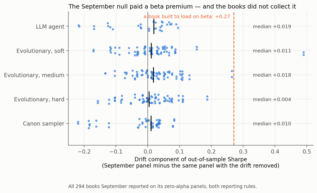
Every book September reported, on the published panel and on its drift-free twin

So September’s headline — that a research agent manufactures an in-sample Sharpe of 2.1 from nothing, and that 88% of it is explained by two integers in the log — stands. The generator does not. It has been replaced, the arithmetic is in the repository, and the correction is in this post rather than in a footnote, because a null you cannot verify is what this entire post is about.

Setup

The null. Factor-structured daily panels: 400 names, regime-switching volatility on the market and three latent factors, Student-t idiosyncratic shocks, lognormal dispersion in volatility. Zero drift, symmetric clipping, and — the part the September generator got wrong — separate random streams for structure (betas, loadings, volatilities, regime paths) and for innovations, so a fresh path can be drawn through the same world.

Verifying that a null is null is harder than writing one. The pre-registered acceptance test probed a constant-beta book and two oracle signals; it passed on two and, on the third, produced a +0.093 on the sixty study seeds that went away on a 120-seed replication. That episode is in the deviations file, and the acceptance file records the pre-registered failure rather than only the replication that passed. It also convinced me the test was too blunt, so there is a better one: 200 expressions drawn from the signal grammar before any panel existed, of which a median of 184 evaluate cleanly on a given panel, across 40 fresh null panels — 7,346 signal-panels, mean annualised Sharpe +0.017, 95% CI [−0.015, +0.048].

Two honest caveats on that. It is measured on the 1,000-day training window, not on the 2,000-day window the books are scored on. And on the exact sixty seeds this study ran, the residual tilt from the acceptance test is bounded at about +0.09 — larger than several of the out-of-sample numbers below. I flag them where they appear.

The pipeline being controlled. An evolutionary search over the same price-only grammar as the September post — returns, moving averages, rolling moments, range position, rolling beta and correlation, with cross-sectional and time-series normalisations. Twelve rounds of twenty-five expressions. The uncontrolled baseline reports the three highest in-sample Sharpes as an equal-weight book. Sixty seeds (9000–9059); 1,000 training days; 2,000 untouched days for scoring.

The two things worth measuring. Every control is placed on two axes.

How much manufactured Sharpe does it remove? Measured on panels with no alpha, and — this matters more than it sounds — measured on the number a user of that control would actually report. If a gate abstains, nothing is reported. If a control re-selects on a validation window, the researcher reports the validation-window number, not the training number they just threw away. If a control searches a shorter window, the researcher reports the shorter window’s Sharpe. Measuring every control on the original training window, which is what I did in the first pass of this study, flatters every re-selection control enormously and is the single largest correction here.

How much real alpha does it destroy? Measured on the same panels with a signal planted in them. Because each seed’s panels are drawn from identical innovations and differ only in the plant, the same book can be scored on both, which separates the exposure a noise-selected book has to the plant by construction from the gain that selecting on the planted panel actually adds. Only the second is “finding alpha”.

Two plants, and why. My first plant was calibrated to an in-sample Sharpe of about 1.0 — below the 1.77 the search manufactures from noise. A pipeline that ranks on in-sample Sharpe must then prefer the noise, so “the search fails to find real alpha” was a property of my calibration rather than a finding. There are now two, both calibrated on thirty seeds (8000–8029) rather than the three the first pass used: a weak plant and a strong one, with realised out-of-sample oracle Sharpes on the study seeds of 0.59 and 2.43.

The analysis plan, the predictions and the estimators were committed before the first search ran. Eighteen departures from them are logged, including several this study’s reviewers forced.

1. Selection manufactures the Sharpe. The search adds nothing.

Start with the uncontrolled pipeline on panels containing nothing:

Uncontrolled pipeline, 60 null panelsValue
Reported in-sample Sharpe1.77 (SE 0.04)
Realised out-of-sample Sharpe, 2,000 days+0.015 (SE 0.051)
One-way turnover, per day19.5%
Net of 5 bp per unit of turnover, at ≈2.5% book volatility−1.00

Familiar enough. Now the part I did not expect. Take 200 expressions drawn at random from the grammar before any panel is generated — no search, no feedback, no breeding — and keep the best three by in-sample Sharpe. On the same kind of null panel that book has an annualised in-sample Sharpe of 1.99 (SE 0.05, 40 panels).

Put the evolutionary search on exactly the same footing — its own logged candidates, the same 700-day window, the same complete-case filter, top three re-selected on that window — and it reports 1.95 (SE 0.05, 60 panels). The difference is 0.04, Welch t = 0.60.

Twelve rounds of adaptive search, three hundred evaluations, mutation and crossover, and the machinery adds nothing measurable to the manufactured number. Picking three things out of a hundred and eighty-odd does all of the work. (The two arms run on different seed sets and are not paired; the pools are matched at 182 against 184 candidates after filtering, with participation ratios of 13 and 15.)

Whatever your research process is — an agent, a grid, a graduate student with a notebook — the quantity that produces the fictitious Sharpe is the size of the set you chose from, and nothing clever has to have happened inside.

2. The holdout that made the number bigger

Here is the reported in-sample Sharpe on panels with no alpha, for each control, measured on the window that control actually reports:

ControlReported Sharpe, null panelsManufactured Sharpe removedAbstains
Internal gate (search 750 days, pick on 250)3.08−0.74—
Internal gate + leg cap of 12.45−0.38—
750-day search, no gate2.15−0.22—
Leg cap 121.78−0.01—
Uncontrolled baseline1.77——
Leg cap 11.650.07—
Budget 6 × 251.590.10—
Budget 12 × 121.560.12—
Budget 6 × 121.420.20—
Out-of-path gate (fresh innovations)1.360.23—
CSCV / PBO gate1.080.3925 of 60
Romano–Wolf stepdown0.410.7748 of 60
Deflated Sharpe hurdle0.001.0060 of 60

Read the last column before the middle one. For the three gates, the removal figure is driven by the abstention rate rather than by any reduction: those gates never make a fiction smaller. They make it rarer — and on the panels where Romano–Wolf does pass, the book it lets through reports 2.04, above the 1.77 it was meant to discipline; the PBO gate’s pass-conditional number is 1.85. That is why each gate’s removal figure sits below its abstention rate — 0.77 against 48 abstentions in 60, 0.39 against 25 — and it means that conditional on getting an answer out of them, you get a worse number than if you had not asked.

Now the top of the table. The train/validate split is the most widely practised control in quantitative research, and on a panel with no alpha it made the reported number 74% larger.

The mechanism is not subtle once you see it. On a panel with no alpha, every point of reported Sharpe is selection. The standard error of a Sharpe estimate scales as one over the square root of the sample, and for a fixed candidate pool the expected maximum scales with that standard error — so the ratio of two reported maxima should be the square root of the inverse ratio of their sample sizes. Those sample sizes are the days the Sharpe is actually computed over, after each book’s warm-up is dropped: 876 for the baseline, 591 for the 750-day search, and a clean 250 for the validation window, which needs no warm-up.

Predicted: √(876/591) = 1.2172 and √(876/250) = 1.872. Observed: 1.2175 and 1.742. The first is right to three decimal places. The gate falls a little short of its prediction because it selects from a pool bred on a different window, so its candidates are not the baseline’s candidates.

Look at the “750-day search, no gate” row, which is there precisely to separate the two effects. Running the same shorter search and reporting its own window’s top three already inflates the number by 22%. The gate adds a further 52 points of the baseline on top of that. Splitting the sample does not remove the selection: it relocates the selection to a shorter window, where selection is cheaper and its rewards are larger — and then hands you that number to report. This is the practical form of a result that is already well established in adaptive data analysis: a holdout reused for selection stops being a holdout [8].

The same logic hits the out-of-path gate, which I expected to be the best control in the study. It re-scores every candidate on a genuinely fresh path through the same world and keeps the best three. A top-three-of-two-hundred maximum over 1,000 fresh days is still worth 1.36. The gate does not remove the manufactured Sharpe. It moves it onto a new path and lets you report it there with a clear conscience.

If a control ends by selecting a maximum, the maximum is the problem, and the control has not addressed it.

One anticipation. A 750/250 split is not a straw split — 70/30 and 80/20 are the conventional choices, and the effect gets worse as the validation window shrinks, so a shop splitting 80/20 on four years is further along this curve than the one measured here.

3. The corrections are fine. You are pointing them at the wrong family.

Three of these controls are formal multiple-testing procedures with published guarantees: the deflated Sharpe ratio [1], the CSCV probability of backtest overfitting [2], and a Romano–Wolf stepdown at 5% familywise error [3], bootstrapped with a stationary block bootstrap [4]. Their realised size on null data is well known to be disappointing in practice. The question that seems not to get asked is whether that is the procedure’s fault.

So I measured each twice: once on the family of candidates the search produced, and once on a family of 200 expressions fixed before the data existed.
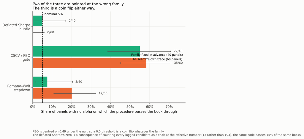
Realised size on a family fixed in advance against the search’s own trace

ProcedureFamily fixed in advance (40 panels)The search’s own trace (60 panels)
Deflated Sharpe hurdle2 of 40 (5%)0 of 60 at N = 193 logged; 9 of 60 (15%) at N effective = 13
CSCV / PBO gate22 of 40 (55%)35 of 60 (58%)
Romano–Wolf stepdown3 of 40 (8%)12 of 60 (20%)

On a family chosen before the data I can detect no inflation in either formal procedure. Forty panels is not enough to certify a 5% test — the Romano–Wolf interval runs from 1.6% to 20.4% — so read that column as the absence of the gross inflation the search family produces, not as a calibration certificate. What is unambiguous is the other side. Pointed at the family the search produced, Romano–Wolf rejects on 12 of 60 panels containing nothing: four times nominal, binomial p < 10⁻⁴. Forty panels against sixty is too little to make the 8%-versus-20% contrast itself significant — Fisher’s exact test on that comparison gives p = 0.15 — so the claim that carries is the one against nominal, not the one across columns. The size inflation on the search family is also not a bootstrap artefact: it holds at expected block lengths of 5, 21 and 63 days and at 500 and 2,000 replications, ranging from 18% to 20% across all four settings.

Why? Not because the bootstrap fails to see the generations that bred the survivors — restrict the family to the search’s round-zero population, random expressions no selection has touched, and rejections fall from 12 panels to 6 (paired exact p = 0.07). That points at adaptive breeding as one contributor rather than the whole story; on sixty panels it is a direction, not a decomposition. The rest is the plainer fact that the family was chosen by looking at the window the test then uses.

The deflated Sharpe ratio is a more uncomfortable case, because its answer is determined by a number you supply. It needs the number of trials; I gave it the count of distinct expressions the search logged, a mean of 193 across panels (range 103 to 258). Those are not independent trials — the participation ratio of their correlation matrix averages 13 (range 5 to 26). Feeding 193 independent trials into a formula that assumes independence pushes the expected-maximum benchmark above the book’s Sharpe on 40 of 60 panels, and leaves the z-statistic short of the 95th percentile on the other twenty — so the hurdle rejects everything. Feed it 13 and the same code, on the same books, passes 9 of 60 — three times nominal (p = 0.003), in the opposite direction. The control’s verdict is a function of a modelling choice nobody documents. To be clear, no published implementation asks for an effective trial count; this is an extension of the method, not a correction to it.

And then there is PBO, which I had been treating as a control and which is not one. CSCV’s logit statistic is symmetric about zero when the candidate strategies are exchangeable and null, so the probability of backtest overfitting is centred on 0.49 — by construction, not by accident. A threshold at 0.5 is therefore a coin flip on data containing nothing: it passes 55% of pre-specified null books and 58% of searched null books. It is not powerless — against the strong plant it passes 95% — but a gate whose false-pass rate is 58% is not a 5% test, whatever it does on real signal.

4. What the controls cost you

Removing fiction is half of a control’s job. The other half is not destroying the thing you are looking for, and you cannot measure that on a null panel.

Against the strong plant — realised out-of-sample oracle Sharpe 2.43, above what the search can manufacture — here is what each control finds of it, alongside what it removes:
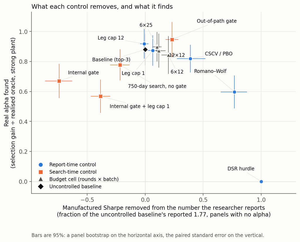
What each control removes and what it keeps

The right-hand column is the selection gain defined in the Setup — what selecting on the planted panel adds over what a null-selected book earns on it by construction. The raw ratio of book Sharpe to oracle is lower, because a book’s exposure to the plant is slightly negative on average: 0.81 for the baseline and 0.85 for the out-of-path gate.

ControlManufactured Sharpe removedReal alpha found (selection gain ÷ oracle)
Out-of-path gate0.230.95
Leg cap 12−0.010.92
Budget 6 × 250.100.90
Uncontrolled baseline—0.88
Leg cap 10.070.87
Budget 12 × 120.120.87
Budget 6 × 120.200.84
CSCV / PBO gate0.390.82
750-day search, no gate−0.220.78
Internal gate−0.740.67
Romano–Wolf stepdown0.770.60
Internal gate + leg cap 1−0.380.57
Deflated Sharpe hurdle1.000.00

The minimum difference detectable at 80% power between the baseline and any of the seven pre-registered controls in that column, after Holm across the whole 84-test scan, runs from 0.05 to 0.21 of the oracle. Differences smaller than that should not be read — including the gap between the out-of-path gate’s 0.95 and the uncontrolled baseline’s 0.88, which is nominally the largest in the table and is not separable at this sample size.

The deflated Sharpe hurdle rejects a genuine 2.4-Sharpe strategy on all sixty panels, and passes exactly one of the sixty carrying the weak plant. Its perfect score in the removal column and its zero in the retention column are the same fact stated twice. A control that abstains on everything is unfalsifiable on null data and useless on real data, and you cannot tell those two properties apart without running a planted arm.

Romano–Wolf is the most defensible trade in the table: it removes 77% of the fiction — by abstaining four times in five — and keeps 60% of a strong real signal. That is a real control with a real price, which is more than most of this column can claim.

The out-of-path gate keeps the most alpha while removing a real 23% of the fiction. It is the only control whose null-panel out-of-sample Sharpe is even marginally negative (−0.086, SE 0.045, 95% CI [−0.17, +0.00]) — a t of 1.9 in a scan across fourteen arms, and inside the residual-tilt bound I flagged in the Setup, so I would not lean on the sign.

Four controls dominate the internal gate on both axes after Holm adjustment: leg cap 1, leg cap 12, the out-of-path gate, and — awkwardly — the PBO gate I have just described as a coin flip. No other pair dominates. That a gate with no size control still dominates the internal gate says more about the internal gate than it does about PBO.

A fourteenth arm, the shorter search with a leg cap of 1, is in the repository and not in these tables: it reports 2.01 on null panels — a little less inflation than the window-matched arm’s 2.15 — and finds 0.78 of the plant, which is the window-matched arm’s figure to within noise.
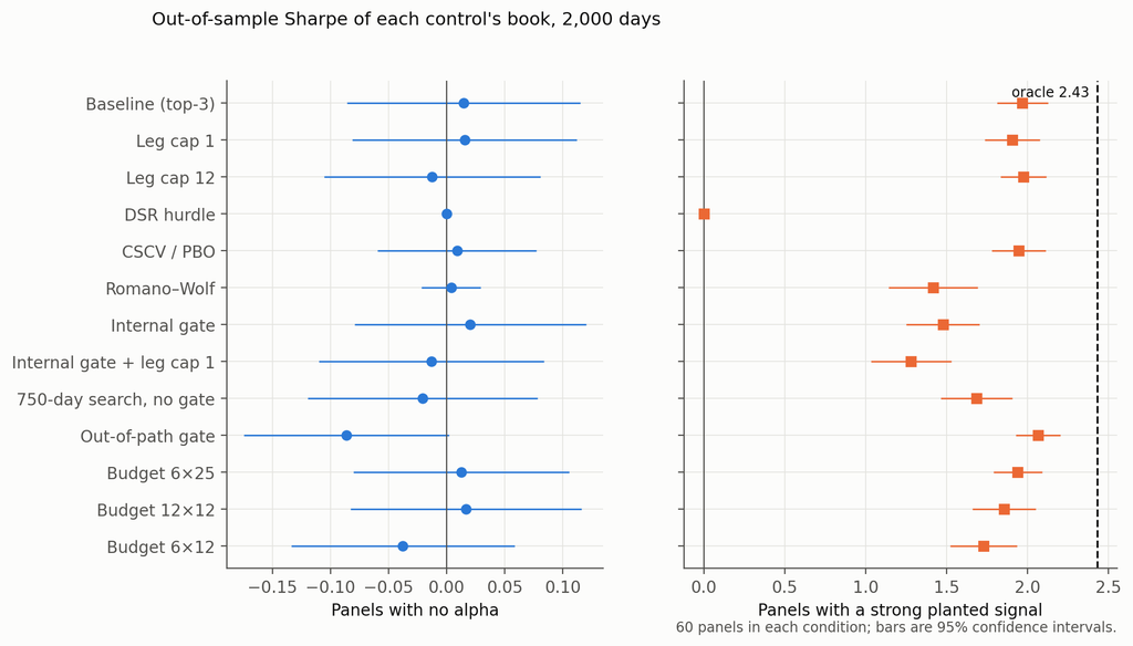
Out-of-sample Sharpe of each control’s book, with no alpha and with a strong plant

One more thing this table only shows because there is a strong plant in the study. Against the weak plant — oracle 0.59 — the uncontrolled pipeline’s selection gain is 11% of the oracle with a minimum detectable effect of 27%. That is not a finding, it is a non-detection, and the first pass of this study reported it as “the search captures 6% of the real signal”. The honest version is conditional and worth stating precisely: a search that ranks on in-sample Sharpe finds real alpha when the real alpha is larger than the alpha it can manufacture, and there is no evidence either way when it is smaller.

5. The agent behaves much like the machine

Eighteen fresh runs of the September research agent through a gated harness, six per condition, with the prompt frozen:

ConditionReported in-sampleRealised out-of-sampleOracleFound the plant
No alpha1.41−0.16 (SE 0.12)——
Weak plant1.52+0.24 (SE 0.17)0.503 of 6 exactly, 4 of 6 by family
Strong plant2.91+2.04 (SE 0.16)2.313 of 6 exactly, 6 of 6 by family

Manufactures on nothing, indistinguishable from noise against a weak signal, and its book earns 88% of the strong plant’s oracle out of sample against the mechanical pipeline’s 81% on the same raw basis. The arms ran on different panels and are not formally compared; qualitatively, whatever an LLM researcher is doing, it is not different enough from an evolutionary search to warrant a different control regime.

The arm is not blinded: the run id the agent types on every harness call carries the condition, K0, K1 or K2. Nothing in the logs refers to it, but it was in front of the agent, and six runs per condition is a small arm.

Two details worth having. The agents worked harder when there was more to find — 4.2 evaluation batches of a permitted 12 against the weak plant, 8.5 against the strong one — but they did not stop early on the null panel, where they used 5.7 batches and one run burned all twelve. That is responsiveness to signal strength, not an ability to notice there is nothing there.

And the twelve September agent traces, re-scored under the report-time controls on drift-free panels, behave as the mechanical arms do: the deflated Sharpe hurdle passes 0 of 12, PBO 5 of 12, Romano–Wolf 7 of 12. The exception is leg caps, which move an agent’s reported Sharpe by +0.02 on average at a cap of one and −0.02 at a cap of twelve — never by more than 0.29 on any single run, and in no consistent direction — because an agent’s legs live inside a single expression rather than in the count of expressions. Any control that counts expressions is close to blind to an agent.

6. One real path, for illustration

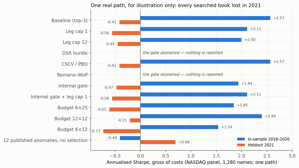
The same pipeline on a real panel — 1,280 NASDAQ names, search 2018–2020, holdout 2021 [5]. One path, a stale and survivorship-conditioned dataset, and a universe filter that looks at the whole sample. It evidences nothing; it is here because it makes the synthetic result legible.

BookIn-sample 2018–2020Holdout 2021Through May 2023
Baseline (top-3)+2.57−0.41−0.24
Leg cap 1+2.11−0.56−0.45
Leg cap 12+2.00−0.45−0.26
CSCV / PBO (passed)+2.57−0.41−0.24
Internal gate+1.94−0.47−0.26
Internal gate + leg cap 1+2.11−0.56−0.45
Budget 6 × 25+1.85−0.61−0.52
Budget 12 × 12+2.40−0.21−0.30
Budget 6 × 12+1.54−0.73−0.64
Deflated Sharpe hurdleabstained——
Romano–Wolfabstained——
Twelve published anomalies, no selection−0.40+0.69+0.69

Every searched book on the real panel, in sample and out

Every searched book turned negative. The unselected canon, which looked worst in sample, was the only thing that worked out of sample. Consistent with the synthetic result, and worth precisely as much as one path is worth.

One inconsistency to flag rather than let a reader find: the in-sample column here is the full 2018–2020 window for every book, including the internal gate, so it is not the reported-window number section 2 corrects to. On this arm the gate therefore appears to lower the in-sample figure when the synthetic result says it raises the number the gate’s user would report. The real panel’s dataset is fetched over the network and I could not re-score that row from the sandbox this study ran in; it is stated here rather than quietly left in the table.

The pre-registration scorecard

PredictionVerdict
P1 the out-of-path gate dominates the DSR hurdle on both axesRefuted, with each control winning one axis: the out-of-path gate removes 1.36 less of the reported Sharpe (CI [−1.45, −1.27]) and finds 2.07 more of the plant (CI [+1.92, +2.21])
P2 a leg cap of 1 removes ≥ 0.20 more than the smallest budget cellRefuted: −0.13, CI [−0.19, −0.07]
P3 the DSR hurdle’s size exceeds 25%Refuted: 0 of 60, conditional on N = logged candidates
P4a the internal gate costs ≥ 0.10 Sharpe on planted panelsConfirmed: −0.49, CI [−0.69, −0.29]
P4b the internal gate removes ≥ 0.50 of the manufactured SharpeRefuted, and in the opposite direction: −0.74

Things that did not work

The leg axis. Capping a book at one leg removes 0.13 less manufactured Sharpe than the smallest search budget does — the budget axis beat the leg axis, and leg caps are close to a no-op on this pipeline. Against an agent they are a complete no-op, for the reason in section 5. This is the one place where I expected a result from the literature to transfer and it didn’t: in-sample statistics do inflate with the number of combined signals [9], but not in a way a cap on the count can reach when the signals are themselves sums.

The pre-registered “oracle frontier” — thresholding candidates on their true out-of-sample Sharpe to trace the best attainable trade-off — is not reported at all. Estimating “true” out-of-sample Sharpe on the same window that scores the books is circular, and on null panels it obligingly produced a frontier that “retained” +0.60 of Sharpe that does not exist. The file is in the repository; the chart does not draw it.

And the first version of this study, which four reviewers took apart before publication. The largest correction was measuring each control on the number a researcher reports rather than the number they discard, which reversed the sign of the headline. The second was noticing that my planted signal had been calibrated to a level the search could beat by fabrication, which made one of my conclusions a property of the experiment rather than of the world. The third was catching three numbers quoted from the weak-plant arm where the text said otherwise. The fourth was showing that this post’s own draft compared the random family and the search on different windows, which inflated the gap in section 1 into a result it is not. All eighteen deviations are logged, and the first-pass tables sit in the repository beside the corrected ones.

What this does and does not show

It does show that on a verified-null panel an in-sample Sharpe of about 1.9 comes out of selecting three candidates from a couple of hundred, on the window the selection is made, and that twelve rounds of adaptive search add nothing measurable to that number.

It does show that a held-out validation window, used the way it is normally used, raises the reported Sharpe rather than lowering it, by roughly the factor the standard error of a Sharpe estimate predicts; and that a fresh-path re-test mostly relocates the manufactured Sharpe rather than removing it.

It does show that two of the three formal procedures show no detectable inflation on a family fixed in advance and are grossly mis-sized on a family the search selected; and that the third is centred on its own threshold under the null and therefore does not decide anything about size.

It does show that a pipeline, mechanical or agentic, recovers most of a planted signal strong enough to beat what it can manufacture — and that the deflated Sharpe hurdle, as conventionally parameterised, destroys all of it.

It does not show that any of these procedures is wrong. Each is implemented here against its published definition and is doing what it was designed to do on the input it is handed.

It does not show anything about faint alpha. Against a signal with a 0.59 oracle Sharpe this design cannot separate “finds nothing” from “finds a quarter of it”. That needs more panels or a longer scoring window.

It does not show a ranking of controls that transfers. The removal axis depends on the reporting convention, the retention axis on a plant that happens to be a single expression the grammar can write exactly — evaluated verbatim by the mechanical search on only 6 of the 60 strong-plant panels, so its findability is not an artefact of expressibility, but a plant the grammar cannot write at all would give a different answer. The leg-cap results depend on a grammar in which a leg is a separate expression, and every net-of-cost number on a book volatility of about 2.5%.

It does not show anything about real markets. One path on a stale dataset is an illustration.

So what do you do?

Report the number you selected on, and say which window it is. Most of the apparent power of every re-selection control in this study came from measuring it on a window the researcher had already discarded: the out-of-path gate’s removal falls from 0.99 to 0.23 when you do this properly, and the internal gate’s flips sign, from +0.47 to −0.74. If your validation split produces a Sharpe of 3.1 where your in-sample fit produced 1.8, the honest headline is 3.1, and the fact that it is larger should alarm you rather than reassure you.

Write down the family before you look. Not the trial count — the family. Every procedure in section 3 shows no inflation on a family fixed in advance and gross inflation on a family your search selected, and the difference between those is a decision you make before the data, not a correction you apply after it.

If you use the deflated Sharpe ratio, state how you counted trials, and report the effective number alongside the raw count. The gap between 193 and 13 on the same candidate set moved the pass rate from 0% to 15%. No published implementation asks for an effective count, so this is an extension rather than a fix — but a DSR quoted without saying how trials were counted is a number with a free parameter in it.

Stop using a PBO threshold of 0.5 as a gate. It is centred on 0.49 under the null. Use the distribution, or use something else.

Run a planted arm. This is the one that costs real effort and is worth it. A control that abstains on everything looks perfect on a null panel; you only find out what it costs when you give it something real to find. And calibrate the plant above what your own pipeline can fabricate, or you will measure your calibration rather than your control — which is exactly what the first version of this study did.

Code and data

The repository holds the pre-registered analysis plan committed before the first run, eighteen logged deviations from it, the corrected generator with its bitwise verification against the September panels, the calibration of both plants, the full study across 180 panels, the pre-specified-family placebo, the erratum arithmetic against all 294 previously published books, the agent harness with every run log and journal, the canary tests, and the analysis and figure code. Seeds: study panels 9000–9059, calibration 8000–8029, placebo panels 9500–9539, pre-specified family drawn from seed 20260921. Everything except the LLM calls reproduces from those seeds; the LLM calls are not re-runnable, which is why the logs are included in full. The repository is at github.com/jkinlay/research-controls; this article refers to commit c11241e.

Two requests of anyone re-running it. Fix your family before you look at the data, and keep the list. And run a planted arm alongside the null arm — half the results here are invisible without one.

References

[1] Bailey & López de Prado, The Deflated Sharpe Ratio: Correcting for Selection Bias, Backtest Overfitting and Non-Normality, Journal of Portfolio Management 40(5), 2014.

[2] Bailey, Borwein, López de Prado & Zhu, The Probability of Backtest Overfitting, Journal of Computational Finance 20(4), 2017; and Pseudo-Mathematics and Financial Charlatanism, Notices of the AMS 61(5), 2014, for the expected-maximum-Sharpe result.

[3] Romano & Wolf, Stepwise Multiple Testing as Formalized Data Snooping, Econometrica 73(4), 2005, 1237–1282. The stepdown implemented here is the one-sided studentised version at 5% familywise error.

[4] Politis & Romano, The Stationary Bootstrap, Journal of the American Statistical Association 89(428), 1994. Expected block length 21 days throughout. The section 3 size result is stable across that choice: 18% at a block length of 5, 20% at 21, 18% at 63, and 18% at 21 with 2,000 replications rather than 500.

[5] skfolio, load_nasdaq_dataset — daily adjusted closes, 1,455 NASDAQ constituents, 2018-01-02 to 2023-05-31, documented by its authors as a stale dataset not intended for investment or commercial use. Filtered here to 1,280 names with median price ≥ $5.

[6] Harvey & Liu, Backtesting, Journal of Portfolio Management 42(1), 2015 — the multiple-testing haircut the report-time controls in section 3 descend from.

[7] Harvey & Liu, False (and Missed) Discoveries in Financial Economics, Journal of Finance 75(5), 2020, on the two-sided cost of correction; section 4 is a direct measurement of the missed-discovery side. See also Chen, The Limits of p-Hacking: Some Thought Experiments, Journal of Finance 76(5), 2021, 2447–2480, for the argument that selection alone cannot account for the observed cross-section — the complement of the measurement in section 1.

[8] Dwork, Feldman, Hardt, Pitassi, Reingold & Roth, The reusable holdout: Preserving validity in adaptive data analysis, Science 349(6248), 2015. Section 2 is the practical, one-reuse form of the result that a holdout used for selection stops being a holdout.

[9] Novy-Marx, Backtesting Strategies Based on Multiple Signals, NBER Working Paper 21329, 2015, on the inflation of in-sample statistics with the number of combined signals — the leg axis that section 4 finds to be a no-op here.

Disclosure: I run systematic strategies. Nothing here is a recommendation, and no strategy discussed is one I trade. These are diagnostic quantities from a methodological experiment on synthetic data and one stale public dataset, not a track record.


Robustness in Quantitative Research and Trading

What is Strategy Robustness?  What is its relevance to Quantitative Research and Trading?

One of the most highly desired properties of any financial model or investment strategy, by investors and managers alike, is robustness.  I would define robustness as the ability of the strategy to deliver a consistent  results across a wide range of market conditions.  It, of course, by no means the only desirable property – investing in Treasury bills is also a pretty robust strategy, although the returns are unlikely to set an investor’s pulse racing – but it does ensure that the investor, or manager, is unlikely to be on the receiving end of an ugly surprise when market conditions adjust.

Robustness is not the same thing as low volatility, which also tends to be a characteristic highly prized by many investors.  A strategy may operate consistently, with low volatility in certain market conditions, but behave very differently in other.  For instance, a delta-hedged short-volatility book containing exotic derivative positions.   The point is that empirical researchers do not know the true data-generating process for the markets they are modeling. When specifying an empirical model they need to make arbitrary assumptions. An example is the common assumption that assets returns follow a Gaussian distribution.  In fact, the empirical distribution of the great majority of asset process exhibit the characteristic of “fat tails”, which can result from the interplay between multiple market states with random transitions.  See this post for details:

http://jonathankinlay.com/2014/05/a-quantitative-analysis-of-stationarity-and-fat-tails/


In statistical arbitrage, for example, quantitative researchers often make use of cointegration models to build pairs trading strategies.  However the testing procedures used in current practice are not sufficient powerful to distinguish between cointegrated processes and those whose evolution just happens to correlate temporarily, resulting in the frequent breakdown in cointegrating relationships.  For instance, see this post:

http://jonathankinlay.com/2017/06/statistical-arbitrage-breaks/

Modeling Assumptions are Often Wrong – and We Know It

We are, of course, not the first to suggest that empirical models are misspecified:

“All models are wrong, but some are useful” (Box 1976, Box and Draper 1987).


Martin Feldstein (1982: 829): “In practice all econometric specifications are necessarily false models.”


Luke Keele (2008: 1): “Statistical models are always simplifications, and even the most complicated model will be a pale imitation of reality.”


Peter Kennedy (2008: 71): “It is now generally acknowledged that econometric models are false and there is no hope, or pretense, that through them truth will be found.”

During the crash of 2008 quantitative Analysts and risk managers found out the hard way that the assumptions underpinning the copula models used to price and hedge credit derivative products were highly sensitive to market conditions.  In other words, they were not robust.  See this post for more on the application of copula theory in risk management:

http://jonathankinlay.com/2017/01/copulas-risk-management/


Robustness Testing in Quantitative Research and Trading

We interpret model misspecification as model uncertainty. Robustness tests analyze model uncertainty by comparing a baseline model to plausible alternative model specifications.  Rather than trying to specify models correctly (an impossible task given causal complexity), researchers should test whether the results obtained by their baseline model, which is their best attempt of optimizing the specification of their empirical model, hold when they systematically replace the baseline model specification with plausible alternatives. This is the practice of robustness testing.

SSALGOTRADING AD

Robustness testing analyzes the uncertainty of models and tests whether estimated effects of interest are sensitive to changes in model specifications. The uncertainty about the baseline model’s estimated effect size shrinks if the robustness test model finds the same or similar point estimate with smaller standard errors, though with multiple robustness tests the uncertainty likely increases. The uncertainty about the baseline model’s estimated effect size increases of the robustness test model obtains different point estimates and/or gets larger standard errors. Either way, robustness tests can increase the validity of inferences.

Robustness testing replaces the scientific crowd by a systematic evaluation of model alternatives.

Robustness in Quantitative Research

In the literature, robustness has been defined in different ways:

  • as same sign and significance (Leamer)
  • as weighted average effect (Bayesian and Frequentist Model Averaging)
  • as effect stability We define robustness as effect stability.

Parameter Stability and Properties of Robustness

Robustness is the share of the probability density distribution of the baseline model that falls within the 95-percent confidence interval of the baseline model.  In formulaeic terms:

Formula

  • Robustness is left-–right symmetric: identical positive and negative deviations of the robustness test compared to the baseline model give the same degree of robustness.
  • If the standard error of the robustness test is smaller than the one from the baseline model, ρ converges to 1 as long as the difference in point estimates is negligible.
  • For any given standard error of the robustness test, ρ is always and unambiguously smaller the larger the difference in point estimates.
  • Differences in point estimates have a strong influence on ρ if the standard error of the robustness test is small but a small influence if the standard errors are large.

Robustness Testing in Four Steps

  1. Define the subjectively optimal specification for the data-generating process at hand. Call this model the baseline model.
  2. Identify assumptions made in the specification of the baseline model which are potentially arbitrary and that could be replaced with alternative plausible assumptions.
  3. Develop models that change one of the baseline model’s assumptions at a time. These alternatives are called robustness test models.
  4. Compare the estimated effects of each robustness test model to the baseline model and compute the estimated degree of robustness.

Model Variation Tests

Model variation tests change one or sometimes more model specification assumptions and replace with an alternative assumption, such as:

  • change in set of regressors
  • change in functional form
  • change in operationalization
  • change in sample (adding or subtracting cases)

Example: Functional Form Test

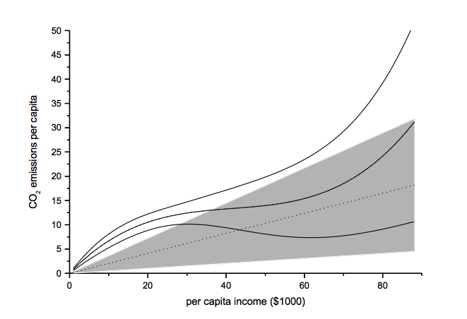
The functional form test examines the baseline model’s functional form assumption against a higher-order polynomial model. The two models should be nested to allow identical functional forms. As an example, we analyze the ‘environmental Kuznets curve’ prediction, which suggests the existence of an inverse u-shaped relation between per capita income and emissions.

Emissions and percapitaincome

Note: grey-shaded area represents confidence interval of baseline model

Another example of functional form testing is given in this review of Yield Curve Models:

http://jonathankinlay.com/2018/08/modeling-the-yield-curve/

Random Permutation Tests

Random permutation tests change specification assumptions repeatedly. Usually, researchers specify a model space and randomly and repeatedly select model from this model space. Examples:

  • sensitivity tests (Leamer 1978)
  • artificial measurement error (Plümper and Neumayer 2009)
  • sample split – attribute aggregation (Traunmüller and Plümper 2017)
  • multiple imputation (King et al. 2001)

We use Monte Carlo simulation to test the sensitivity of the performance of our Quantitative Equity strategy to changes in the price generation process and also in model parameters:

http://jonathankinlay.com/2017/04/new-longshort-equity/

Structured Permutation Tests

Structured permutation tests change a model assumption within a model space in a systematic way. Changes in the assumption are based on a rule, rather than random.  Possibilities here include:

  • sensitivity tests (Levine and Renelt)
  • jackknife test
  • partial demeaning test

Example: Jackknife Robustness Test

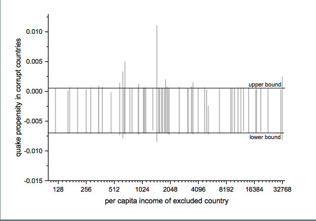
The jackknife robustness test is a structured permutation test that systematically excludes one or more observations from the estimation at a time until all observations have been excluded once. With a ‘group-wise jackknife’ robustness test, researchers systematically drop a set of cases that group together by satisfying a certain criterion – for example, countries within a certain per capita income range or all countries on a certain continent. In the example, we analyse the effect of earthquake propensity on quake mortality for countries with democratic governments, excluding one country at a time. We display the results using per capita income as information on the x-axes.

jackknife

Upper and lower bound mark the confidence interval of the baseline model.

Robustness Limit Tests

Robustness limit tests provide a way of analyzing structured permutation tests. These tests ask how much a model specification has to change to render the effect of interest non-robust. Some examples of robustness limit testing approaches:

  • unobserved omitted variables (Rosenbaum 1991)
  • measurement error
  • under- and overrepresentation
  • omitted variable correlation

For an example of limit testing, see this post on a review of the Lognormal Mixture Model:

http://jonathankinlay.com/2018/08/the-lognormal-mixture-variance-model/

Summary on Robustness Testing

Robustness tests have become an integral part of research methodology. Robustness tests allow to study the influence of arbitrary specification assumptions on estimates. They can identify uncertainties that otherwise slip the attention of empirical researchers. Robustness tests offer the currently most promising answer to model uncertainty.

Futures WealthBuilder

We are launching a new product, the Futures WealthBuilder,  a CTA system that trades futures contracts in several highly liquid financial and commodity markets, including SP500 EMinis, Euros, VIX, Gold, US Bonds, 10-year and five-year notes, Corn, Natural Gas and Crude Oil.  Each  component strategy uses a variety of machine learning algorithms to detect trends, seasonal effects and mean-reversion.  We develop several different types of model for each market, and deploy them according to their suitability for current market conditions.

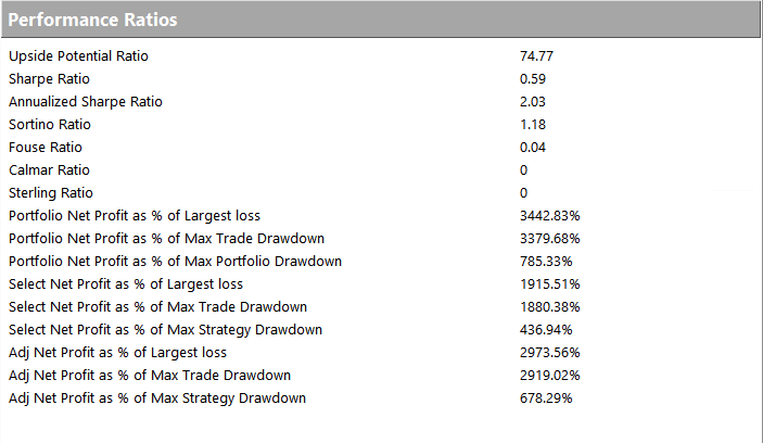
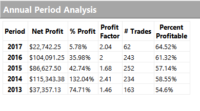
Performance of the strategy (net of fees) since 2013 is detailed in the charts and tables below.  Notable features include a Sharpe Ratio of just over 2, an annual rate of return of 190% on an account size of $50,000, and a maximum drawdown of around 8% over the last three years.  It is worth mentioning, too, that the strategy produces approximately equal rates of return on both long and short trades, with an overall profit factor above 2.


Fig1


Fig2


Fig3

Fig4


Fig5

Low Correlation

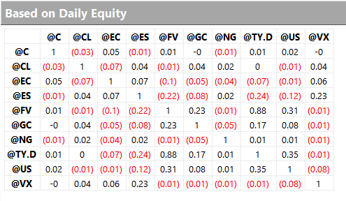
Despite a high level of correlation between several of the underlying markets, the correlation between the component strategies of Futures WealthBuilder are, in the majority of cases, negligibly small (with a few exceptions, such as the high correlation between the 10-year and 5-year note strategies).  This accounts for the relative high level of return in relation to portfolio risk, as measured by the Sharpe Ratio.   We offer strategies in both products chiefly as a mean of providing additional liquidity, rather than for their diversification benefit.

Fig 6

Strategy Robustness

Strategy robustness is a key consideration in the design stage.  We use Monte Carlo simulation to evaluate scenarios not seen in historical price data in order to ensure consistent performance across the widest possible range of market conditions.  Our methodology introduces random fluctuations to historical prices, increasing or decreasing them by as much as 30%.  We allow similar random fluctuations in that value strategy parameters, to ensure that our models perform consistently without being overly-sensitive to the specific parameter values we have specified.  Finally, we allow the start date of each sub-system to vary randomly by up to a year.

The effect of these variations is to produce a wide range of outcomes in terms of strategy performance.  We focus on the 5% worst outcomes, ranked by profitability, and select only those strategies whose performance is acceptable under these adverse scenarios.  In this way we reduce the risk of overfitting the models while providing more realistic expectations of model performance going forward.  This procedure also has the effect of reducing portfolio tail risk, and the maximum peak-to-valley drawdown likely to be produced by the strategy in future.
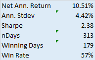
GC Daily Stress Test

Futures WealthBuilder on Collective 2

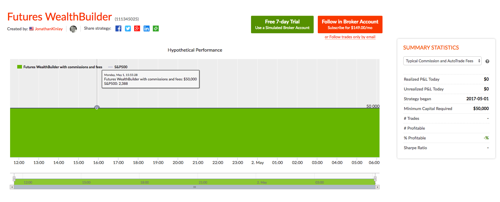
We will be running a variant of the Futures WealthBuilder strategy on the Collective 2 site, using a subset of the strategy models in several futures markets(see this page for details).  Subscribers will be able to link and auto-trade the strategy in their own account, assuming they make use of one of the approved brokerages which include Interactive Brokers, MB Trading and several others.

Obviously the performance is unlikely to be as good as the complete strategy, since several component sub-strategies will not be traded on Collective 2.  However, this does give the subscriber the option to trial the strategy in simulation before plunging in with real money.

Fig7


The Internal Bar Strength Indicator

Internal Bar Strength (IBS) is an idea that has been around for some time.  IBS is based on the position of the day’s close in relation to the day’s range: it takes a value of 0 if the closing price is the lowest price of the day, and 1 if the closing price is the highest price of the day.

More formally:

IBS  =  (Close – Low) / (High – Low)

The IBS effect may be related to intraday over-reaction to news or market movements, which are then ”corrected” the next day.  It serves as a measure of the tendency of a price series to mean-revert over daily horizons.  I use the term “daily” advisedly: so far as I am aware, there has been no research (including my own) demonstrating the existence of an IBS effect at time horizons shorter, or longer, than one day.  Indeed, there has been very little in the way of academic research into the concept of any kind, which is strange considering how compelling are the results it is capable of producing.  Practitioners have been happy enough with that state of affairs, content to deploy this neglected indicator in their trading strategies, where it has often proved to be extremely useful (we use IBS in one of our volatility strategies). Since 2013, however, the cat has been let out of the bag, thanks to an excellent research paper by Alexander Pagonidis, who writes an interesting quantitative finance blog.

The essence of the idea is that stocks that close in the lowest part of the daily range, with an IBS of below, say, 0.2, will tend to rally the next day, while stocks that close in the highest quintile will often decline in value in the following session.  In his paper “The IBS Effect: Mean Reversion in Equity ETFs” (2013), Pagonidis researches the IBS effect in equity index ETFs in the US and several international markets.  He confirms that low IBS values in these assets are associated with high returns in the following day session, while high IBS values are associated with low returns. Average returns when IBS is below 0.20 are .35% ,while average returns when IBS is above 0.80 are -0.13%. According to his research, this effect has been present in equity ETFs since the early 90s and has been highly consistent through time.

SSALGOTRADING AD

IBS Strategy Performance

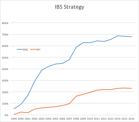
To give the reader some idea of the potential of the IBS effect, I have reproduced below equity curves for the IBS strategy for the SPDR S&P 500 ETF Trust (SPY) and iShares MSCI Singapore ETF (EWS) index ETFs over the period from 1999 to 2016.  The strategy buys at the close when IBS is below 0.2, and sells at the close when IBS exceeds 0.8, liquidating the position at the following market close. Strategy CAGR over the period has been of the order of 13% for SPY and as high as 40% for EWS, ignoring transaction costs.

IBS Strategy Chart SPY EWS


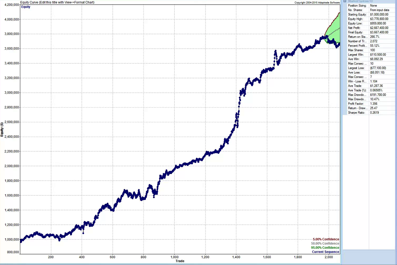
Note that in both cases strategy returns for SPY and EWS have diminished in recent years, turning negative in 2015 and 2016 YTD and this is true for ETFs in general.  It remains to be seen whether this deterioration in strategy performance is temporary or permanent.  There are some indications that the latter holds true, but the evidence is not quite definitive.  For example, the chart below shows daily equity curve for the SPY IBS strategy, with 95% confidence intervals for the latest 100 trades (up to the end of May 2016), constructed using Monte-Carlo bootstrap.  The equity curve appears to have penetrated the lower bound, indicating a statistically significant deterioration in the performance of the IBS strategy for SPY over the last year or so (EWS is similar).  That said, the equity curve does fall inside the boundaries of the 99% confidence interval, so those looking for greater certainty about the possible breakdown of the effect will need to wait a little longer for confirmation.


SPY IBS MSA


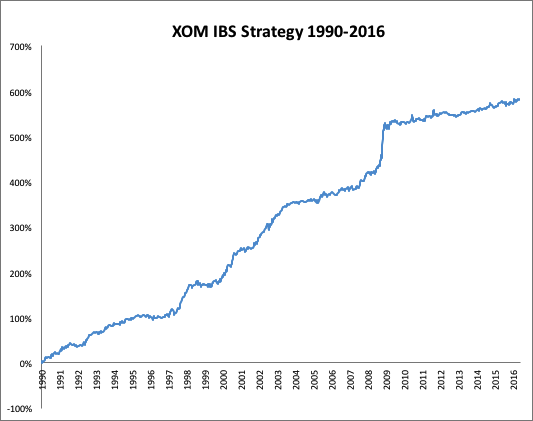
Whatever the outcome may be for SPY and other ETFs going forward, it is certainly true that IBS effects persist strongly for some individual equities, Exxon-Mobil Corp. (XOM) being a case in point (see below).  It’s worth taking note of the exceptional performance of the XOM IBS strategy during the latter quarter of 2008.  I will have much more to say on the application of the IBS indicator for individual equities in a future blog post.


XOM IBS Strategy


The Role of Range, Volume, Bull/Bear Markets, Volatility and Seasonality

Pagonidis goes on to detail several further important findings in relation to IBS.  It is clear from his research that high volatility is related to increased predictability of returns and a more powerful IBS effect, in particular the high IBS-negative return aspect.  As might be expected, the effect is also larger after days with high range, both for high and low IBS extremes.

Volume turns out to be especially important for  U.S. index ETFs:  in fact, the IBS effect only appears to work on high-volume days.

Pagonidis also separates the data into bull and bear market environments, based on whether 200-day returns are positive or not.  The size of the effect is roughly similar in each environment (slightly larger in bear markets), but it is greater in the direction of the overall trend: high IBS readings are followed by larger negative returns during bear markets, and vice versa.

Day of Week Effect

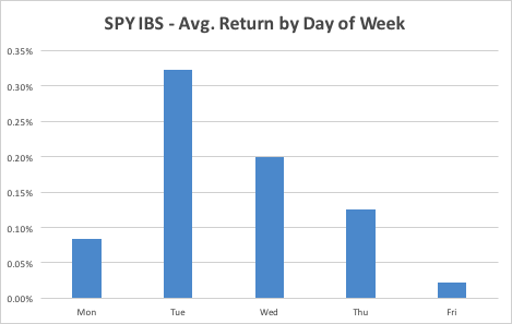
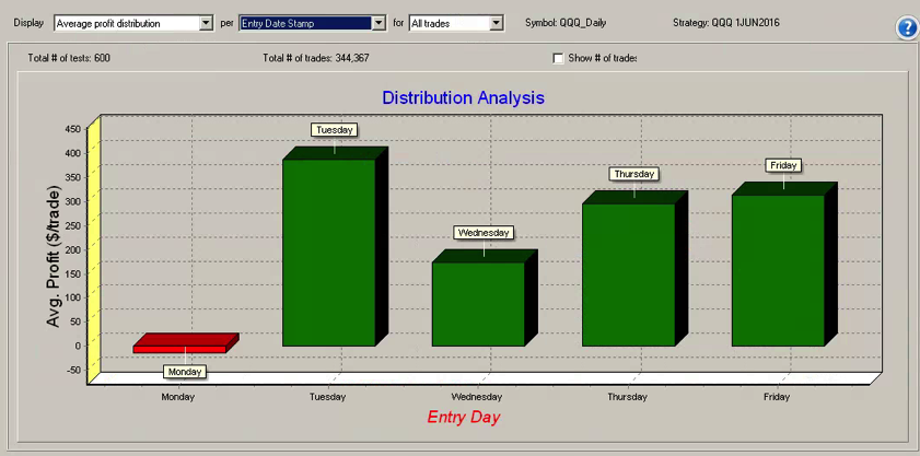
The IBS effect is also strongly seasonal, having the greatest impact on returns from Monday’s close to Tuesday’s close, as illustrated for the SPY ETF in the chart below.  This accounts for the phenomenon known popularly as “Turnaround Tuesday”, i.e. the tendency for the market to recover strongly from losses on a Monday.  The day-of-week effect is weakest for Fridays.


SPY DOW


The mean of the returns distribution is not the only aspect that IBS can predict. Skewness also varies significantly between IBS buckets, with low IBS readings being followed by highly skewed returns, and vice versa. Close-to-close returns after a bottom-bucket IBS day have average skewness of 0.65 across Equity Index ETF products, while top-bucket IBS days are followed by returns with skewness of 0.03. This finding has very useful risk management applications for investors concerned with tail risk.

IBS as a Filter for a Swing Trading Strategy in QQQ

The returns to an IBS-only strategy are both statistically and economically significant. However, commissions will greatly decrease the returns and increase the maximum drawdowns, however, making such an approach challenging in the real world. One alternative is to combine the IBS effect with mean reversion on longer timescales and only take trades when they align.
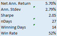
Pagonidis offers a simple demonstration using the Cutler’s RSI indicator that shows how the IBS effect can be used to boost returns of a swing trading strategy while significantly decreasing the number of trades needed.

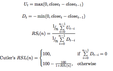
Cutler’s RSI at time t is calculated as follows:


RSI


Pagonidis tests a simple, long-only strategy that trades the PowerShares QQQ Trust, Series 1 (QQQ) ETF using the Cutler’s RSI(3) indicator:

• Go long at the close if RSI(3) < 10

• Maintain the position while RSI(3) ≤ 40

 filter these returns by adding an additional rule based on the value of IBS:

• Enter or maintain long position only if IBS ≤ 0.5

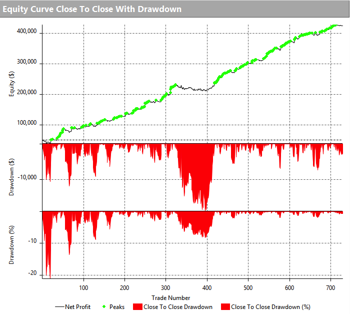
Pangonis claims that the strategy produces rather promising results that “easily beats commissions”;  however, my own rendition of the strategy, assuming commissions of $0.005 per share and slippage of a further $0.02 per share produces results that are distinctly less encouraging:

EC0


Pef0

Strategy Code

For those interested, the code is as follows:

Inputs:
RSILen(3),
RSI_Entry(10),
RSI_Exit(40),
IBS_Threshold(0.5),
Initial_Capital(100000);
Vars:
nShares(100),
RSIval(0),
IBS(0);
RSIval=RSI(C,RSILen);
IBS = (C-L)/(H-L);

nShares = Round(Initial_Capital / Close,0);

If Marketposition = 0 and RSIval > RSI_Entry and IBS < IBS_Threshold then begin
Buy nShares contracts next bar at market;
end;
If Marketposition > 0 and ((RSIval > RSI_Exit) or (IBS_Threshold > IBS_Threshold)) then begin
Sell next bar at market;
end;

Strategy Optimization and Robustness Testing

One can further improve performance by optimizing the trading system parameters, using Tradestation’s excellent Walk Forward Optimization (WFO) module.  This allows us to examine the effect of re-calibrating the strategy parameters are regular intervals, testing the optimized model on out-of-sample data sets of various sizes.  WFO can be used, not only optimize a strategy, but also to examine the sensitivity of its performance to changes in the levels of key parameters.  For example, in the case of the QQQ swing trading strategy, we find that profitability increases monotonically with the length of the RSI indicator, and this effect is especially marked when an IBS threshold level of 0.2 is used:

Sensitivity


Likewise we can test the consistency of the day-of-the-week effect over several OS data sets of  varying size and these tests are consistent with the pattern seen earlier for the IBS indicator, confirming its role as a filter rule in enhancing system profitability:

Distribution Analysis


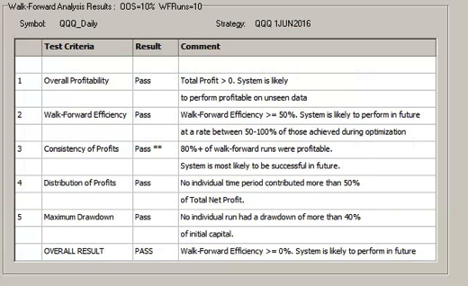
A model that is regularly re-calibrated using WFO is subjected to a series of tests designed to ensure its robustness and consistency in live trading.   The tests include the following:


WFO


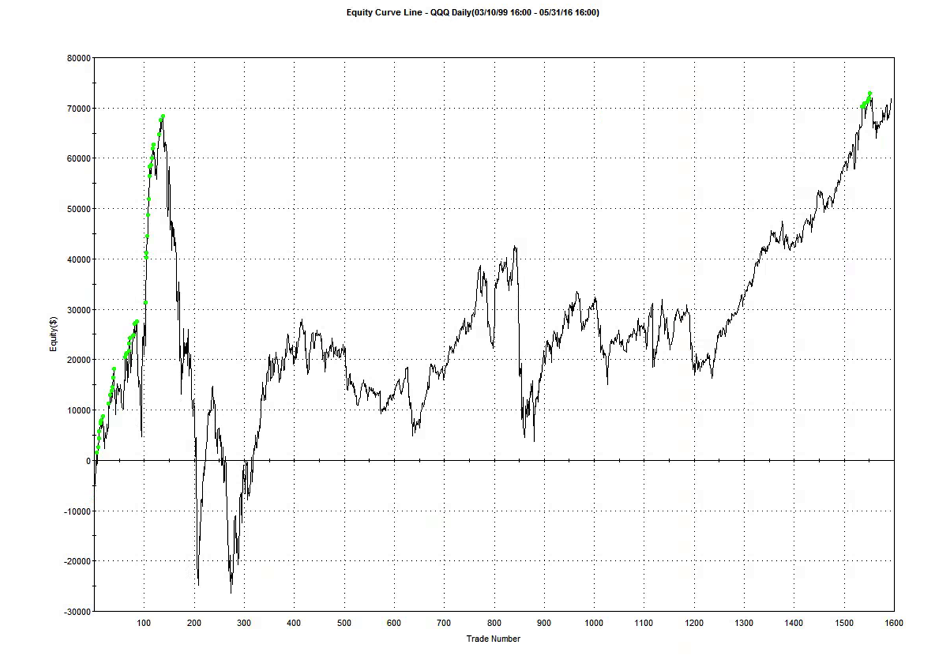
In order to achieve an overall pass rating, the system is required to pass all five tests of its out-of-sample performance, from which Tradestation deems it likely that the system will continue to perform well in live trading.  The results from this procedure appear much more promising than the strategy in its original form, as can be seen from the performance table and equity curve chart shown below.

EC1

Perf1


However, these results include both in-sample and out-of-sample periods.  An examination of the results from the WFO indicate that the overall efficiency of the strategy is around 55%, meaning that the P&L produced by the system in out-of-sample periods amounts to a little over one half of the rate of profit produced during in-sample periods.  Going forward, therefore, we might expect the performance of the system in live trading to be only around half as good as shown here.  While this is still superior to the original system, it may not be considered good enough.  Nonetheless, for the purpose of illustrating the benefits of the IBS indicator as a trade filter, it makes the point.

Another interesting example of an IBS-based trading strategy in the QQQ and SPY ETFs can be found in the following blog post.

Conclusion

Internal Bar Strength is a powerful mean-reversion indicator for equity products traded at daily frequencies, with a consistent effect that has continued from the 1990s through to the current decade. IBS can be used on its own in mean-reversion strategies that have worked well for both US equities and US and International equity index ETFs, or used as a trade filter when combined with other alpha signals.

While there is evidence of a weakening of the IBS effect since around 2013 this is not yet confirmed statistically (at the 99% confidence level) and may simply be the result of normal statistical variation in its efficacy.


A New Approach to Equity Valuation

How Analysts Traditionally Value Equity

fig1I learned the traditional method for producing equity valuations in the 1980’s, from  Chase bank’s excellent credit training program.  The standard technique was to develop several years of projected financial statements, and then discount the cash flows and terminal value to arrive at an NPV. I’m guessing the basic approach hasn’t changed all that much over the last 30-40 years and probably continues to serve as the fundamental building block for M&A transactions and PE deals.

Damadoran

Amongst several excellent texts on the topic I can recommend, for example, Aswath Damodaran’s book on valuation.

Arguably the weakest point in the methodology are the assumptions made about the long term growth rate of the business and the rate used to discount the cash flows to produce the PV.  Since we are dealing with long term projections, small variations in these rates can make a considerable difference to the outcome.

The Monte Carlo Approach

Around 20 years ago I wrote a paper titled “A New Approach to Equity Valuation”, in which I attempted to define a new methodology for equity valuation.  The idea was simple enough:  instead of guessing an appropriate rate to discount the projected cash flows generated by the company, you embed the riskiness into the cash flows themselves, using probability distributions.  That allows you to model the cash flows using Monte Carlo simulation and discount them using the risk-free rate, which is much easier to determine.  In a similar vein,  the model can allow for stochastic growth rates, perhaps also taking into account the arrival of potential new entrants, or disruptive technologies.

I recall taking the idea to an acquaintance of mine who at the time was head of M&A at a prestigious boutique bank in London.  About five minutes into the conversation I realized I had lost him at “Monte Carlo”.  It was yet another instance of the gulf between the fundamental and quantitative approach to investment finance, something I have always regarded as rather artificial.  The line has blurred in several places over the last few decades – option theory of the firm and factor models, to name but two examples – but remains largely intact.  I have met very few equity analysts who have the slightest clue about quantitative research and vice-versa, for that matter.  This is a pity in my view, as there is much to be gained by blending knowledge of the two disciplines.

SSALGOTRADING AD

The basic idea of the Monte Carlo approach is to formulate probability distributions for key variables that drive the business, such as sales, gross margin, cost of goods, etc., as well as related growth rates. You then determine the outcome in terms of P&L and cash flows over a large number of simulations, from which you can derive a probability distribution for the firm/equity value.

npv

There are two potential sources of data one can use to build a Monte Carlo model: the historical distributions of the variables and information from line management. It is the latter that is likely to be especially useful, because you can embed management’s expertise and understanding of the business and its competitive environment directly into the model variables, rather than relying upon a single discount rate to account for all the possible sources of variation in the cash flows.

It can get a little complicated, of course: one cannot simply assume that all the variables evolve independently – COGS is likely to fall as a % of sales as sales increase, for example, due to economies of scale. Such interactive effects are critically important and it is necessary to dig deep into the inner workings of the business to model them successfully.  But to those who may view such a task as overwhelmingly complicated I can offer several counter examples.  For instance, in the 1970’s  I worked on large scale simulation models of the North Sea oil fields that incorporated volumes of information from geology to engineering to financial markets.  Another large scale simulation was built to assess how best to manage tanker traffic at one of the world’s busiest sea ports.

Creating a simulation model of  the financials of a single firm is a simple task, by comparison. And, after you have built the model it will typically remain fundamentally unchanged in basic form for many years making the task of producing valuation estimates much easier in future.

Applications of Monte Carlo Methods in Equity Valuation

Ok, so what’s the point?  At the end of the day, don’t you just end up with the same result as from traditional methods, i.e. an estimate of the equity or firm value? Actually no – what you have instead is an estimate of the probability distribution of the value, something decidedly more useful.

For example:

Contract Negotiation

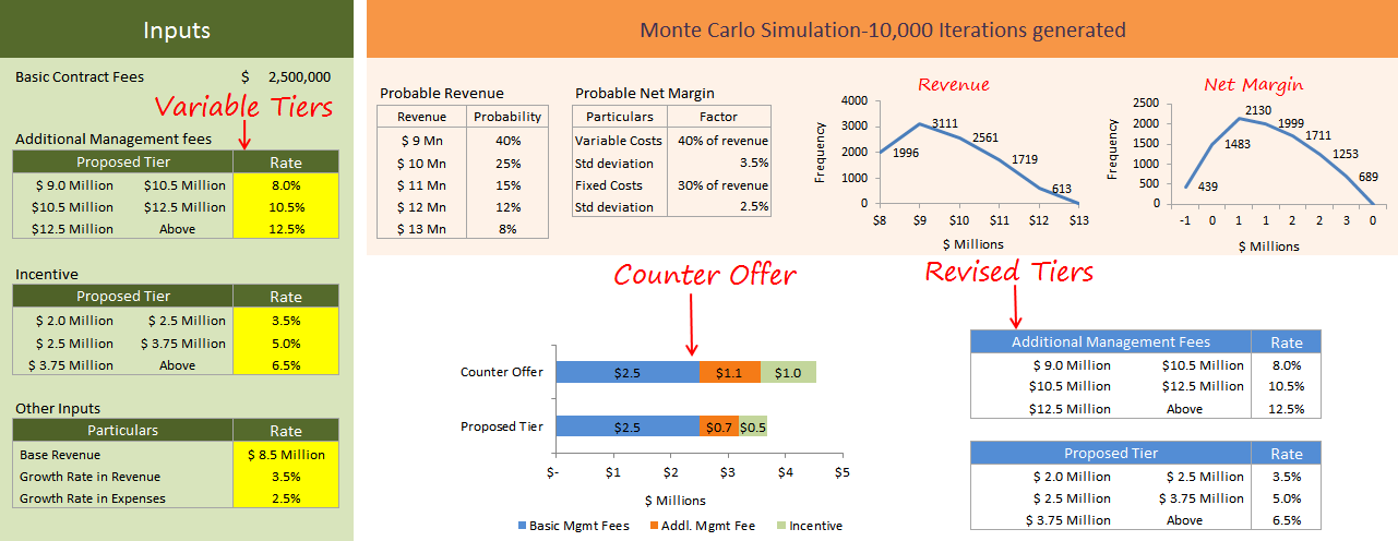
Monte Carlo methods have been applied successfully to model contract negotiation scenarios, for instance for management consulting projects, where several rounds of negotiation are often involved in reaching an agreed pricing structure.

Negotiation

 Stock Selection

You might build a portfolio of value stocks whose share price is below the median value, in the expectation that the majority of the universe will prove to be undervalued, over the long term.  Or you might embed information about the expected value of the equities in your universe (and their cashflow volatilities) into you portfolio construction model.

Private Equity / Mergers & Acquisitions

In a PE or M&A negotiation your model provides a range of values to select from, each of which is associated with an estimated “probability of overpayment”.  For example, your opening bid might be a little below the median value, where it is likely that you are under-bidding for the projected cash flows.  That allows some headroom to increase the bid, if necessary, without incurring too great a risk of over-paying.

Recent Research

A survey of recent research in the field yields some interesting results, amongst them a paper by Magnus Pedersen entitled Monte Carlo Simulation in Financial Valuation (2014).  Pedersen takes a rather different approach to applying Monte Carlo methods to equity valuation.   Specifically, he uses the historical distribution of the price/book ratio to derive the empirical distribution of the equity value rather than modeling the individual cash flows.  This is a sensible compromise for someone who, unlike an analyst at a major sell-side firm, may not have access to management information necessary to build a more sophisticated model.  Nevertheless, Pedersen is able to demonstrate quite interesting results using MC methods to construct equity portfolios (weighted according to the Kelly criterion), in an accompanying paper Portfolio Optimization & Monte Carlo Simulation (2014).

For those who find the subject interesting, Pedersen offers several free books on his web site, which are worth reviewing.

cover_strategies-sp500

Is Your Trading Strategy Still Working?

The Challenge of Validating Strategy Performance

One of the challenges faced by investment strategists is to assess whether a strategy is continuing to perform as it should.  This applies whether it is a new strategy that has been backtested and is now being traded in production, or a strategy that has been live for a while.
All strategies have a limited lifespan.  Markets change, and a trading strategy that can’t accommodate that change will get out of sync with the market and start to lose money. Unless you have a way to identify when a strategy is no longer in sync with the market, months of profitable trading can be undone very quickly.

The issue is particularly important for quantitative strategies.  Firstly, quantitative strategies are susceptible to the risk of over-fitting.  Secondly, unlike a strategy based on fundamental factors, it may be difficult for the analyst to verify that the drivers of strategy profitability remain intact.

Savvy investors are well aware of the risk of quantitative strategies breaking down and are likely to require reassurance that a period of underperformance is a purely temporary phenomenon.

It might be tempting to believe that you will simply stop trading when the strategy stops working.  But given the stochastic nature of investment returns, how do you distinguish a losing streak from a system breakdown?

SSALGOTRADING AD

Stochastic Process Control

One approach to the problem derives from the field of Monte Carlo simulation and stochastic process control.  Here we random draw samples from the distribution of strategy returns and use these to construct a prediction envelope to forecast the range of future returns.  If the equity curve of the strategy over the forecast period  falls outside of the envelope, it would raise serious concerns that the strategy may have broken down.  In those circumstances you would almost certainly want to trade the strategy in smaller size for a while to see if it recovers, or even exit the strategy altogether it it does not.

I will illustrate the procedure for the long/short ETF strategy that I described in an earlier post, making use of Michael Bryant’s excellent Market System Analyzer software.

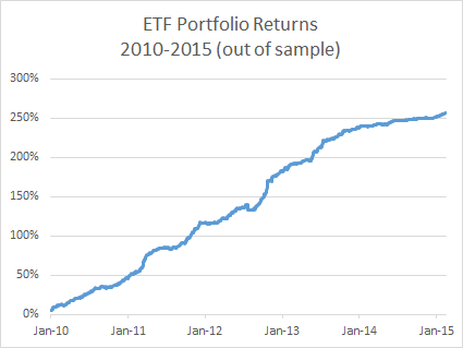
To briefly refresh, the strategy is built using cointegration theory to construct long/short portfolios is a selection of ETFs that provide exposure to US and international equity, currency, real estate and fixed income markets.  The out of sample back-test performance of the strategy is very encouraging:

Fig 2


Fig 1

There was evidently a significant slowdown during 2014, with a reduction in the risk-adjusted returns and win rate for the strategy:

Fig 1

This period might itself have raised questions about the continuing effectiveness of the strategy.  However, we have the benefit of hindsight in seeing that, during the first two months of 2015, performance appeared to be recovering.

Consequently we put the strategy into production testing at the beginning of March 2015 and we now wish to evaluate whether the strategy is continuing on track.   The results indicate that strategy performance has been somewhat weaker than we might have hoped, although this is compensated for by a significant reduction in strategy volatility, so that the net risk-adjusted returns remain somewhat in line with recent back-test history.

Fig 3

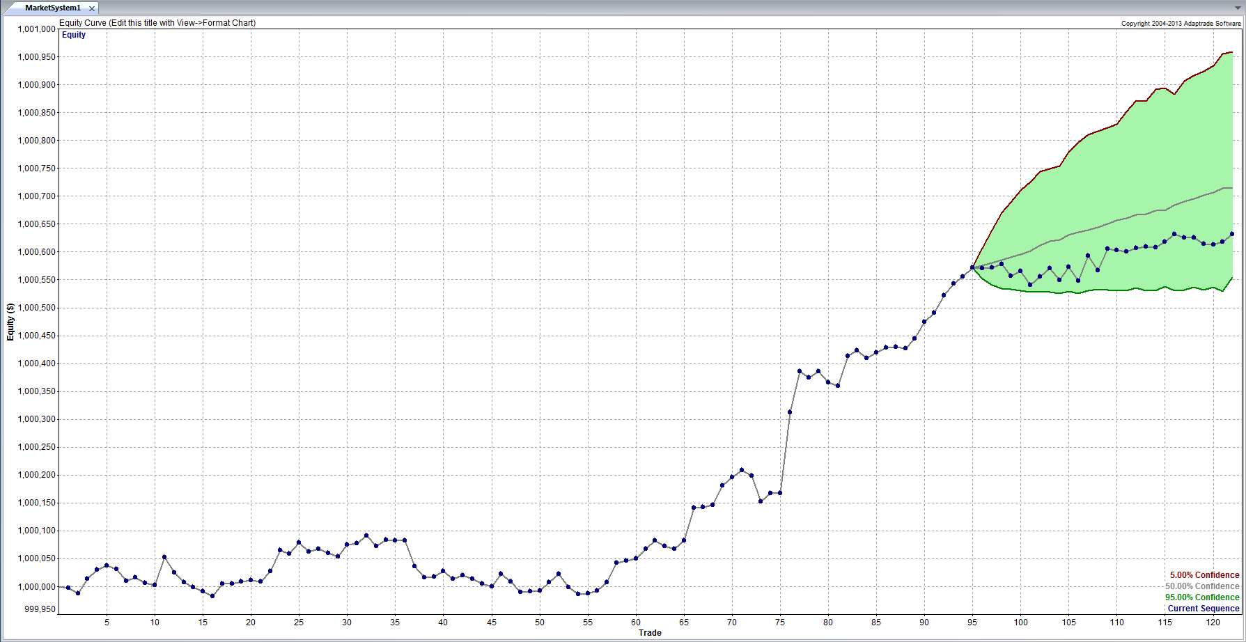
Using the MSA software we sample the most recent back-test returns for the period to the end of Feb 2015, and create a 95% prediction envelope for the returns since the beginning of March, as follows:

Fig 2

As we surmised, during the production period the strategy has slightly underperformed the projected median of the forecast range, but overall the equity curve still falls within the prediction envelope.  As this stage we would tentatively conclude that the strategy is continuing to perform within expected tolerance.

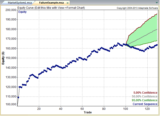
Had we seen a pattern like the one shown in the chart below, our conclusion would have been very different.

Fig 4

As shown in the illustration, the equity curve lies below the lower boundary of the prediction envelope, suggesting that the strategy has failed. In statistical terms, the trades in the validation segment appear not to belong to the same statistical distribution of trades that preceded the validation segment.

This strategy failure can also be explained as follows: The equity curve prior to the validation segment displays relatively little volatility. The drawdowns are modest, and the equity curve follows a fairly straight trajectory. As a result, the prediction envelope is fairly narrow, and the drawdown at the start of the validation segment is so large that the equity curve is unable to rise back above the lower boundary of the envelope. If the history prior to the validation period had been more volatile, it’s possible that the envelope would have been large enough to encompass the equity curve in the validation period.

 CONCLUSION

Systematic trading has the advantage of reducing emotion from trading because the trading system tells you when to buy or sell, eliminating the difficult decision of when to “pull the trigger.” However, when a trading system starts to fail a conflict arises between the need to follow the system without question and the need to stop following the system when it’s no longer working.

Stochastic process control provides a technical, objective method to determine when a trading strategy is no longer working and should be modified or taken offline. The prediction envelope method extrapolates the past trade history using Monte Carlo analysis and compares the actual equity curve to the range of probable equity curves based on the extrapolation.

Next we will look at nonparametric distributions tests  as an alternative method for assessing strategy performance.