Market Noise and Alpha Signals
One of the perennial problems in designing trading systems is noise in the data, which can often drown out an alpha signal. This is turn creates difficulties for a trading system that relies on reading the signal, resulting in greater uncertainty about the trading outcome (i.e. greater volatility in system performance). According to academic research, a great deal of market noise is caused by trading itself. There is apparently not much that can be done about that problem: sure, you can trade after hours or overnight, but the benefit of lower signal contamination from noise traders is offset by the disadvantage of poor liquidity. Hence the thrust of most of the analysis in this area lies in the direction of trying to amplify the signal, often using techniques borrowed from signal processing and related engineering disciplines.
There is, however, one trick that I wanted to share with readers that is worth considering. It allows you to trade during normal market hours, when liquidity is greatest, but at the same time limits the impact of market noise.

Quantifying Market Noise
How do you measure market noise? One simple approach is to start by measuring market volatility, making the not-unreasonable assumption that higher levels of volatility are associated with greater amounts of random movement (i.e noise). Conversely, when markets are relatively calm, a greater proportion of the variation is caused by alpha factors. During the latter periods, there is a greater information content in market data – the signal:noise ratio is larger and hence the alpha signal can be quantified and captured more accurately.
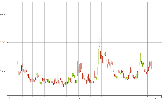
For a market like the E-Mini futures, the variation in daily volatility is considerable, as illustrated in the chart below. The median daily volatility is 1.2%, while the maximum value (in 2008) was 14.7%!
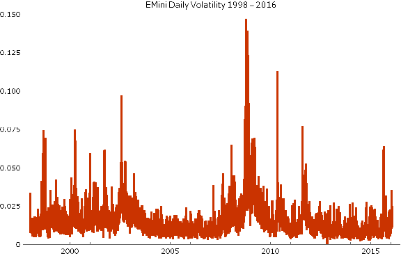
The extremely long tail of the distribution stands out clearly in the following histogram plot.
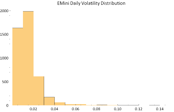
Obviously there are times when the noise in the process is going to drown out almost any alpha signal. What if we could avoid such periods?
Noise Reduction and Model Fitting
Let’s divide our data into two subsets of equal size, comprising days on which volatility was lower, or higher, than the median value. Then let’s go ahead and use our alpha signal(s) to fit a trading model, using only data drawn from the lower volatility segment.
This is actually a little tricky to achieve in practice: most software packages for time series analysis or charting are geared towards data occurring at equally spaced points in time. One useful trick here is to replace the actual date and time values of the observations with sequential date and time values, in order to fool the software into accepting the data, since there are no longer any gaps in the timestamps. Of course, the dates on our time series plot or chart will be incorrect. But that doesn’t matter: as long as we know what the correct timestamps are.
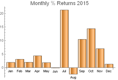
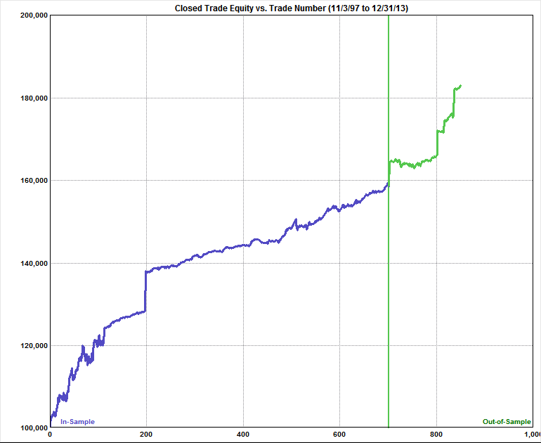
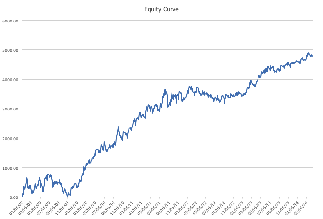
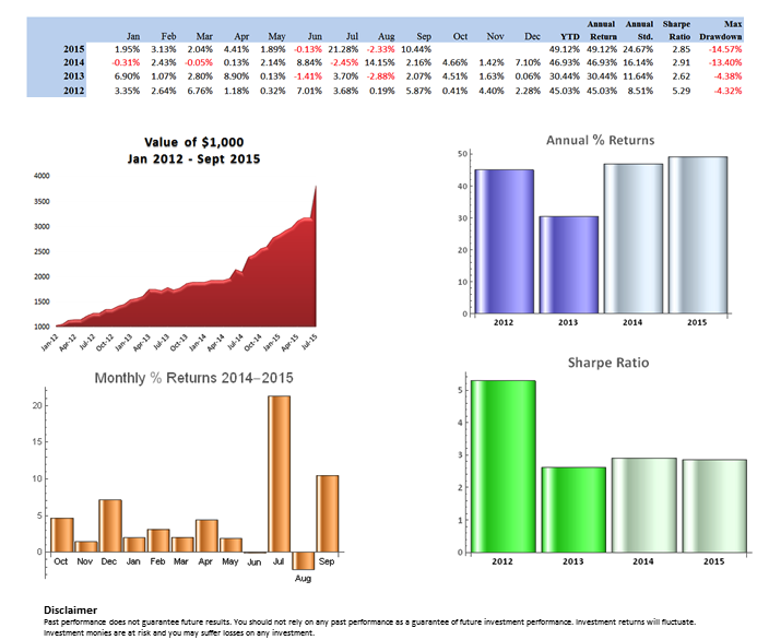
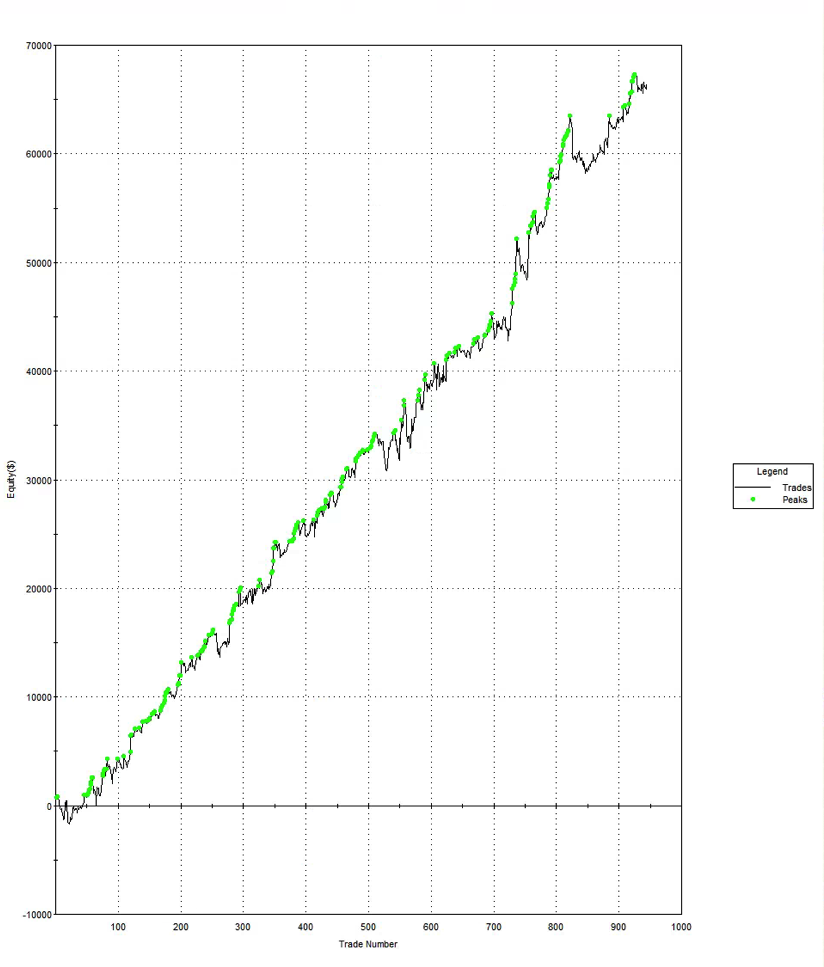
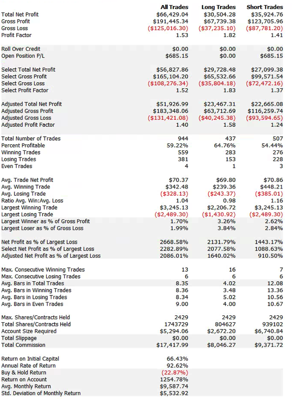
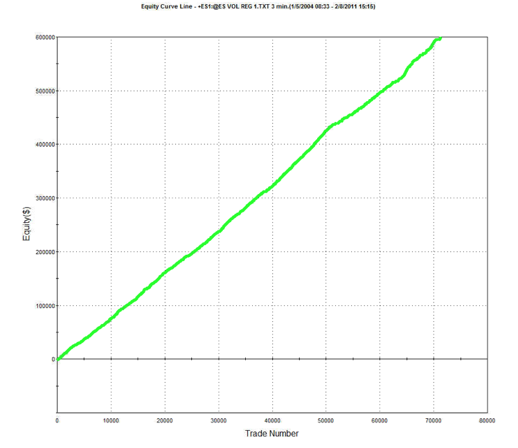
An example of such a system is illustrated below. The model was fitted to 3-Min bar data in EMini futures, but only on days with market volatility below the median value, in the period from 2004 to 2015. The strategy equity curve is exceptionally smooth, as might be expected, and the performance characteristics of the strategy are highly attractive, with a 27% annual rate of return, profit factor of 1.58 and Sharpe Ratio approaching double-digits.

Dealing with the Noisy Trading Days
Let’s say you have developed a trading system that works well on quiet days. What next? There are a couple of ways to go:
(i) Deploy the model only on quiet trading days; stay out of the market on volatile days; or
(ii) Develop a separate trading system to handle volatile market conditions.
Which approach is better? It is likely that the system you develop for trading quiet days will outperform any system you manage to develop for volatile market conditions. So, arguably, you should simply trade your best model when volatility is muted and avoid trading at other times. Any other solution may reduce the overall risk-adjusted return. But that isn’t guaranteed to be the case – and, in fact, I will give an example of systems that, when combined, will in practice yield a higher information ratio than any of the component systems.
Deploying the Trading Systems
The astute reader is likely to have noticed that I have “cheated” by using forward information in the model development process. In building a trading system based only on data drawn from low-volatility days, I have assumed that I can somehow know in advance whether the market is going to be volatile or not, on any given day. Of course, I don’t know for sure whether the upcoming session is going to be volatile and hence whether to deploy my trading system, or stand aside. So is this just a purely theoretical exercise? No, it’s not, for the following reasons.
The first reason is that, unlike the underlying asset market, the market volatility process is, by comparison, highly predictable. This is due to a phenomenon known as “long memory”, i.e. very slow decay in the serial autocorrelations of the volatility process. What that means is that the history of the volatility process contains useful information about its likely future behavior. [There are several posts on this topic in this blog – just search for “long memory”]. So, in principle, one can develop an effective system to forecast market volatility in advance and hence make an informed decision about whether or not to deploy a specific model.
But let’s say you are unpersuaded by this argument and take the view that market volatility is intrinsically unpredictable. Does that make this approach impractical? Not at all. You have a couple of options:
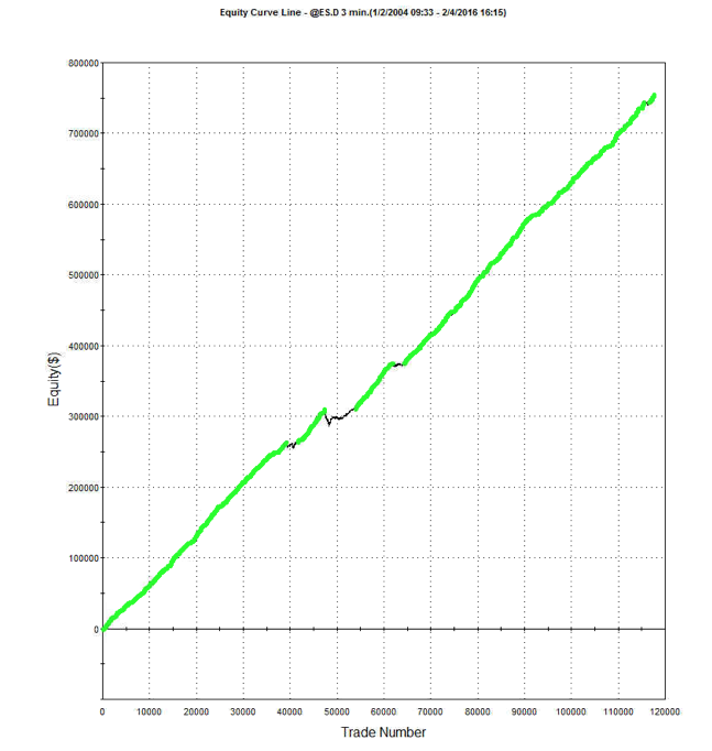
You can test the model built for quiet days on all the market data, including volatile days. It may perform acceptably well across both market regimes.
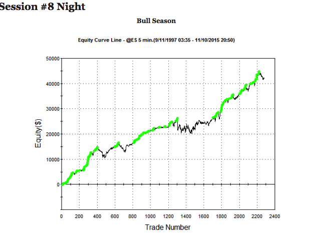
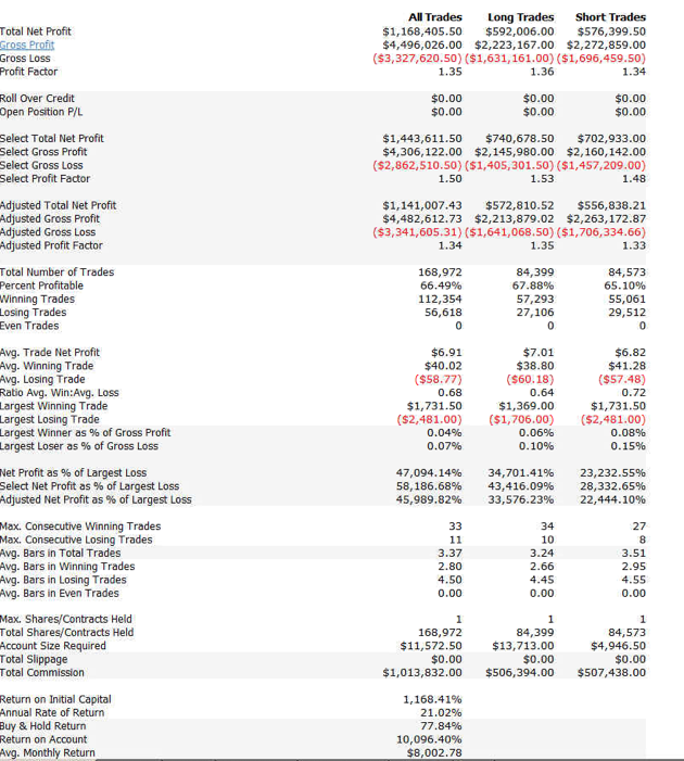
For example, here are the results of a backtest of the model described above on all the market data, including volatile and quiet periods, from 2004-2015. While the performance characteristics are not quite as good, overall the strategy remains very attractive.

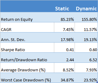
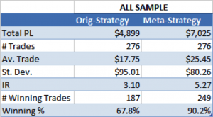
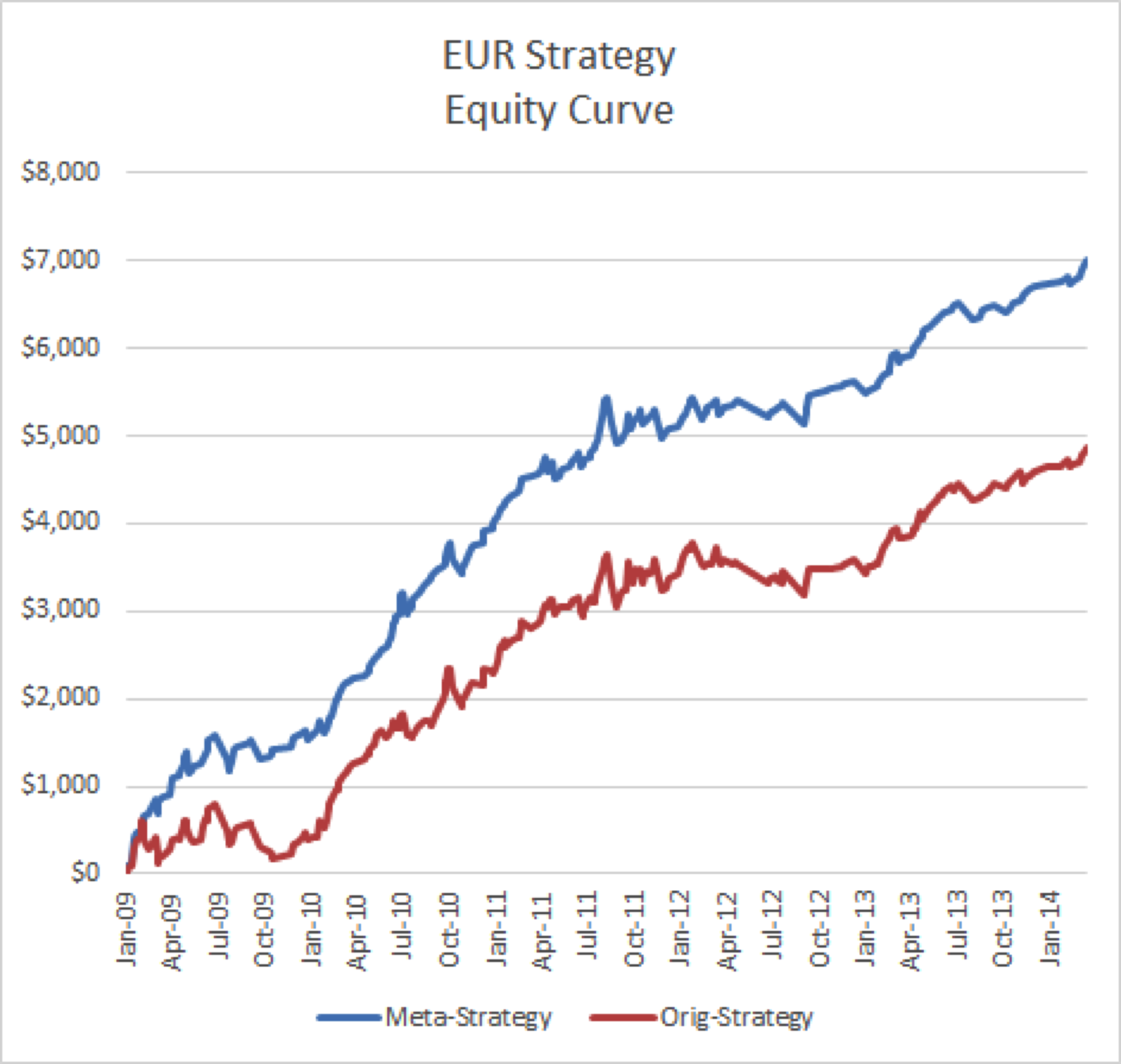
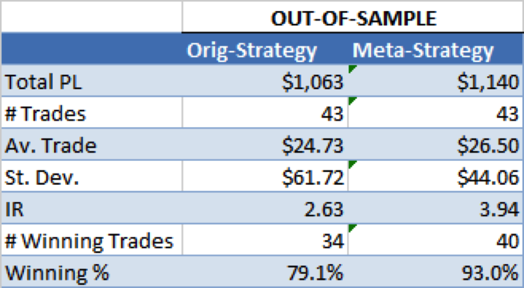
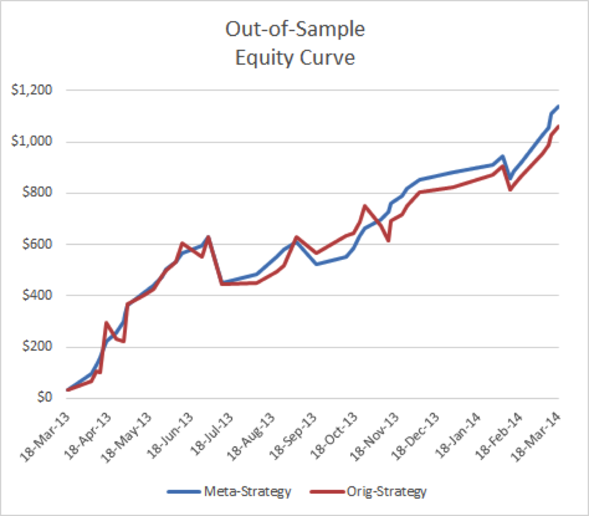
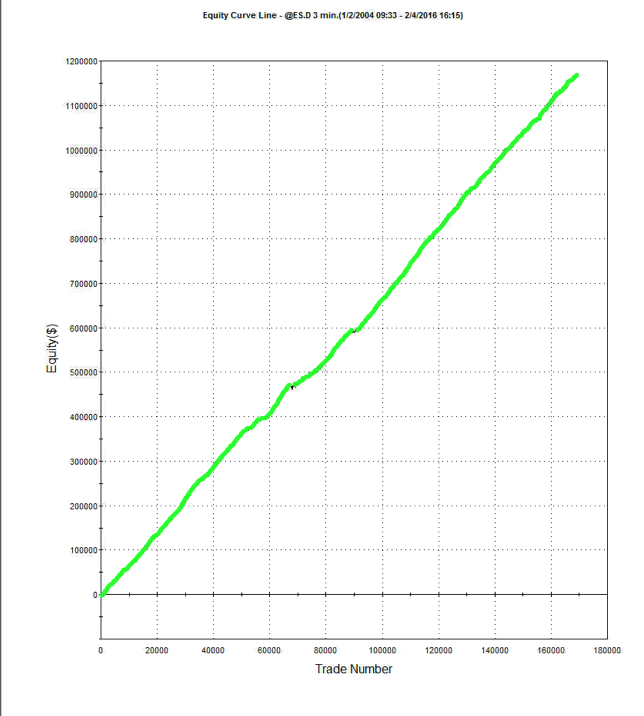
Another approach is to develop a second model for volatile days and deploy both low- and high-volatility regime models simultaneously. The trading systems will interact (if you allow them to) in a highly nonlinear and unpredictable way. It might turn out badly – but on the other hand, it might not! Here, for instance, is the result of combining low- and high-volatility models simultaneously for the Emini futures and running them in parallel. The result is an improvement (relative to the low volatility model alone), not only in the annual rate of return (21% vs 17.8%), but also in the risk-adjusted performance, profit factor and average trade.
CONCLUSION
Separating the data into multiple subsets representing different market regimes allows the system developer to amplify the signal:noise ratio, increasing the effectiveness of his alpha factors. Potentially, this allows important features of the underlying market dynamics to be captured in the model more easily, which can lead to improved trading performance.
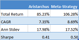
Models developed for different market regimes can be tested across all market conditions and deployed on an everyday basis if shown to be sufficiently robust. Alternatively, a meta-strategy can be developed to forecast the market regime and select the appropriate trading system accordingly.
Finally, it is possible to achieve acceptable, or even very good results, by deploying several different models simultaneously and allowing them to interact, as the market moves from regime to regime.