Market Timing
In an earlier article, I discussed how investors can enhance returns through the strategic use of market timing techniques to step out of the market during difficult conditions.
To emphasize the impact of market timing on investment returns, I have summarized in the chart below how a $1,000 investment would have grown over the 25-year period from July 1990 to June 2014. In the baseline scenario, we assume that the investment is made in a fund that tracks the S&P 500 Index and held for the full term. In the second scenario, we look at the outcome if the investor had stepped out of the market during the market downturns from March 2000 to Feb 2003 and from Jan 2007 to Feb 2009.
Fig. 1: Value of $1,000 Jul 1990-Jun 2014 – S&P 500 Index with and without Market Timing
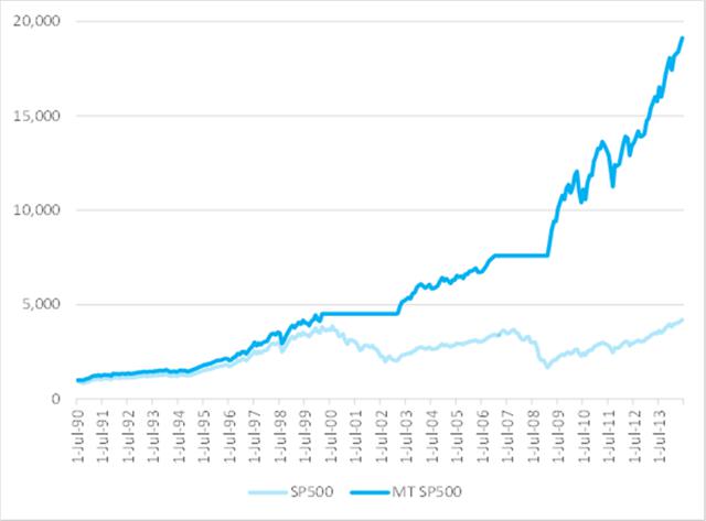
Source: Yahoo Finance, 2014
After 25 years, the investment under the second scenario would have been worth approximately 5x as much as in the baseline scenario. Of course, perfect market timing is unlikely to be achievable. The best an investor can do is employ some kind of market timing indicator, such as the CBOE VIX index, as described in the previous article.
Equity Long Short
For those who mistrust the concept of market timing or who wish to remain invested in the market over the long term regardless of short-term market conditions, an alternative exists that bears consideration.
The equity long/short strategy, in which the investor buys certain stocks while shorting others, is a concept that reputedly originated with Alfred Jones in the 1940s. A long/short equity portfolio seeks to reduce overall market exposure, while profiting from stock gains in the long positions and price declines in the short positions. The idea is that the investor’s equity investments in the long positions are hedged to some degree against a general market decline by the offsetting short positions, from which the concept of a hedge fund is derived.

There are many variations on the long/short theme. Where the long and short positions are individually matched, the strategy is referred to as pairs trading. When the portfolio composition is structured in a way that the overall market exposure on the short side equates to that of the long side, leaving zero net market exposure, the strategy is typically referred to as market-neutral. Variations include dollar-neutral, where the dollar value of aggregate long and short positions is equalized, and beta-neutral, where the portfolio is structured in a way to yield a net zero overall market beta. But in the great majority of cases, such as, for example, in 130/30 strategies, there is a residual net long exposure to the market. Consequently, for the most part, long/short strategies are correlated with the overall market, but they will tend to outperform long-only strategies during market declines, while underperforming during strong market rallies.
Modern Portfolio Theory
Theories abound as to the best way to construct equity portfolios. The most commonly used approach is mean-variance optimization, a concept developed in the 1950s by Harry Markovitz (other more modern approaches include, for example, factor models or CVAR – conditional value at risk).
If we plot the risk and expected return of the assets under consideration, in what is referred to as the investment opportunity set, we see a characteristic “bullet” shape, the upper edge of which is called the efficient frontier (See Fig. 2). Assets on the efficient frontier produce the highest level of expected return for a given level of risk. Equivalently, a portfolio lying on the efficient frontier represents the combination offering the best possible expected return for a given risk level. It transpires that for efficient portfolios, the weights to be assigned to individual assets depend only on the volatilities of the individual assets and the correlation between them, and can be determined by simple linear programming. The inclusion of a riskless asset (such as US T-bills) allows us to construct the Capital Market Line, shown in the figure, which is tangent to the efficient frontier at the portfolio with the highest Sharpe Ratio, which is consequently referred to as the Tangency or Optimal Portfolio.
Fig. 2: Investment Opportunity Set and Efficient Frontier
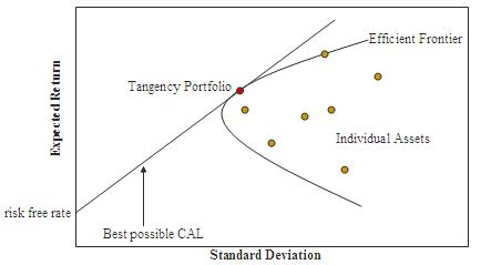
Source: Wikipedia
Paradise Lost
Elegant as it is, MPT is open to challenge as a suitable basis for constructing investment portfolios. The Sharpe Ratio is often an inadequate representation of the investor’s utility function – for example, a strategy may have a high Sharpe Ratio but suffer from large drawdowns, behavior unlikely to be appealing to many investors. Of greater concern is the assumption of constant correlation between the assets in the investment universe. In fact, expected returns, volatilities and correlations fluctuate all the time, inducing changes in the shape of the efficient frontier and the composition of the optimal portfolio, which may be substantial. Not only is the composition of the optimal portfolio unstable, during times of financial crisis, all assets tend to become positively correlated and move down together. The supposed diversification benefit of MPT breaks down when it is needed the most.
I want to spend a little time on these critical issues before introducing a new methodology for portfolio construction. I will illustrate the procedure using a limited investment universe consisting of the dozen stocks listed below. This is, of course, a much more restricted universe than would typically apply in practice, but it does provide a span of different sectors and industries sufficient for our purpose.
| Adobe Systems Inc. (NASDAQ:ADBE) |
| E. I. du Pont de Nemours and Company (NYSE:DD) |
| The Dow Chemical Company (NYSE:DOW) |
| Emerson Electric Co. (NYSE:EMR) |
| Honeywell International Inc. (NYSE:HON) |
| International Business Machines Corporation (NYSE:IBM) |
| McDonald’s Corp. (NYSE:MCD) |
| Oracle Corporation (NYSE:ORCL) |
| The Procter & Gamble Company (NYSE:PG) |
| Texas Instruments Inc. (NASDAQ:TXN) |
| Wells Fargo & Company (NYSE:WFC) |
| Williams Companies, Inc. (NYSE:WMB) |
If we follow the procedure outlined in the preceding section, we arrive at the following depiction of the investment opportunity set and efficient frontier. Note that in the following, the S&P 500 index is used as a proxy for the market portfolio, while the equal portfolio designates a portfolio comprising identical dollar amounts invested in each stock.
Fig. 3: Investment Opportunity Set and Efficient Frontiers for the 12-Stock Portfolio
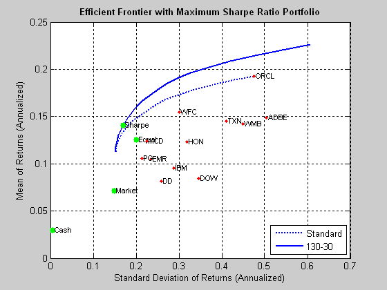
Source: MathWorks Inc.
As you can see, we have derived not one, but two, efficient frontiers. The first is the frontier for standard portfolios that are constrained to be long-only and without use of leverage. The second represents the frontier for 130/30 long-short portfolios, in which we permit leverage of 30%, so that long positions are overweight by a total of 30%, offset by a 30% short allocation. It turns out that in either case, the optimal portfolio yields an average annual return of around 13%, with annual volatility of around 17%, producing a Sharpe ratio of 0.75.
So far so good, but here, of course, we are estimating the optimal portfolio using the entire data set. In practice, we will need to estimate the optimal portfolio with available historical data and rebalance on a regular basis over time. Let’s assume that, starting in July 1995 and rolling forward month by month, we use the latest 60 months of available data to construct the efficient frontier and optimal portfolio.
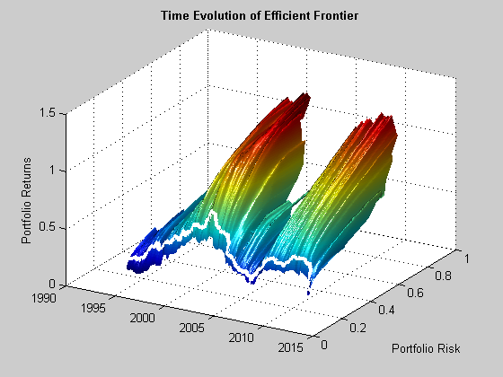
Fig. 4 below illustrates the enormous variation in the shape of the efficient frontier over time, and in the risk/return profile of the optimal long-only portfolio, shown as the white line traversing the frontier surface.
Fig. 4: Time Evolution of the Efficient Frontier and Optimal Portfolio
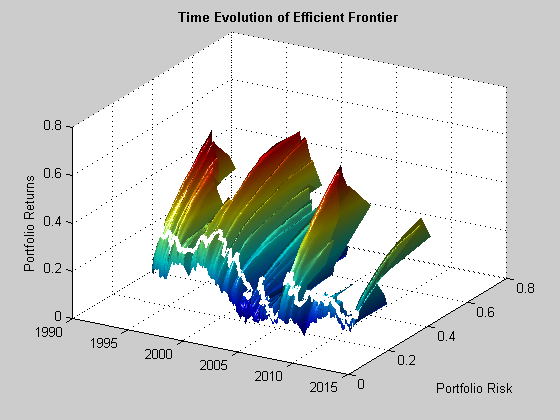
Source: MathWorks Inc.
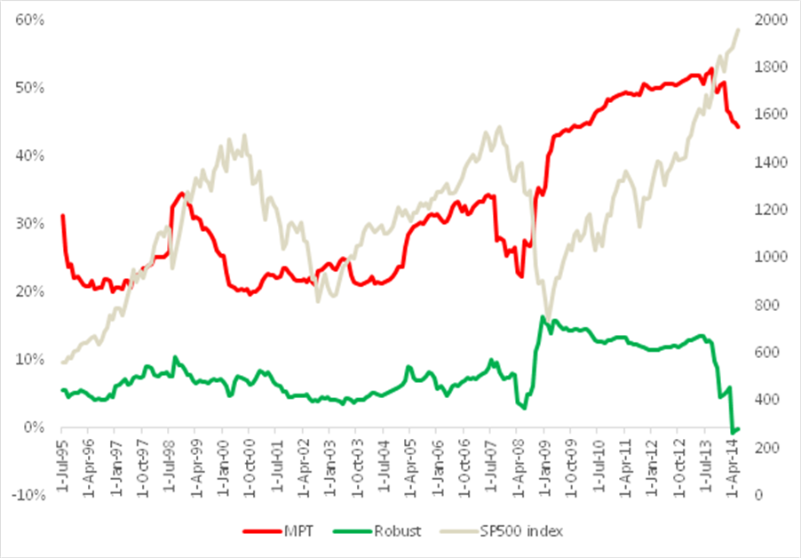
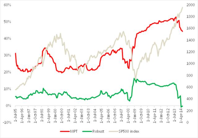
We see in Fig. 5 that the outcome of using the MPT approach is hardly very encouraging: the optimal long-only portfolio underperforms the market both in aggregate, over the entire back-test period, and consistently during the period from 2000-2011. The results for a 130/30 portfolio (not shown) are hardly an improvement, as the use of leverage, if anything, has a tendency to exacerbate portfolio turnover and other undesirable performance characteristics.
Fig. 5: Value of $1,000: Optimal Portfolio vs. S&P 500 Index, Jul 1995-Jun 2014
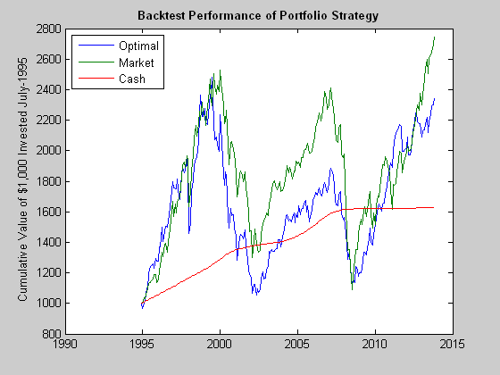
Source: MathWorks Inc.
Part of the reason for the poor performance of the optimal portfolio lies with the assumption of constant correlation. In fact, as illustrated in Fig 6, the average correlation between the monthly returns in the twelve stocks in our universe has fluctuated very substantially over the last twenty years, ranging from a low of just over 20% to a high in excess of 50%, with an annual volatility of 38%. Clearly, the assumption of constant correlation is unsafe.
Fig. 6: Average Correlation, Jul 1995-Jun 2014
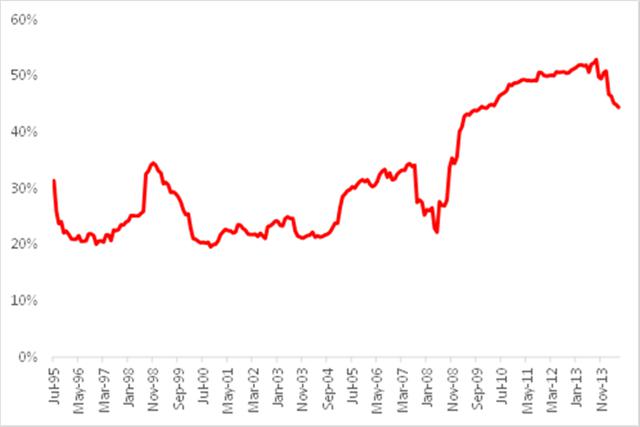
Source: Yahoo Finance, 2014
To add to the difficulties, researchers have found that the out of sample performance of the naïve portfolio, in which equal dollar value is invested in each stock, is typically no worse than that of portfolios constructed using techniques such as mean-variance optimization or factor models1. Due to the difficulty of accurately estimating asset correlations, it would require an estimation window of 3,000 months of historical data for a portfolio of only 25 assets to produce a mean-variance strategy that would outperform an equally-weighted portfolio!
Without piling on the agony with additional concerns about the MPT methodology, such as the assumption of Normality in asset returns, it is already clear that there are significant shortcomings to the approach.
Robust Portfolios
Many attempts have been made by its supporters to address the practical limitations of MPT, while other researchers have focused attention on alternative methodologies. In practice, however, it remains a challenge for any of the common techniques in use today to produce portfolios that will consistently outperform a naïve, equally-weighted portfolio. The approach discussed here represents a radical departure from standard methods, both in its objectives and in its methodology. I will discuss the general procedure without getting into all of the details, some of which are proprietary.
Let us revert for a moment to the initial discussion of market timing at the start of this article. We showed that if only we could time the market and step aside during major market declines, the outcome for the market portfolio would be a five-fold improvement in performance over the period from Aug 1990 to Jun 2014. In one sense, it would not take “much” to produce a substantial uplift in performance: what is needed is simply the ability to avoid the most extreme market drawdowns. We can identify this as a feature of what might be described as a “robust” portfolio, i.e. one with a limited tendency to participate in major market corrections. Focusing now on the general concept of “robustness”, what other characteristics might we want our ideal portfolio to have? We might consider, for example, some or all of the following:
- Ratio of total returns to max drawdown
- Percentage of profitable days
- Number of drawdowns and average length of drawdowns
- Sortino ratio
- Correlation to perfect equity curve
- Profit factor (ratio of gross profit to gross loss)
- Variability in average correlation
The list is by no means exhaustive or prescriptive. But these factors relate to a common theme, which we may characterize as robustness. A portfolio or strategy constructed with these criteria in mind is likely to have a very different composition and set of performance characteristics when compared to an optimal portfolio in the mean-variance sense. Furthermore, it is by no means the case that the robustness of such a portfolio must come at the expense of lower expected returns. As we have seen, a portfolio which only produces a zero return during major market declines has far higher overall returns than one that is correlated with the market. If the portfolio can be constructed in a way that will tend to produce positive returns during market downturns, so much the better. In other words, what we are describing is a long/short portfolio whose correlation to the market adapts to market conditions, having a tendency to become negative when markets are in decline and positive when they are rising.
The first insight of this approach, then, is that we use different criteria, often multi-dimensional, to define optimality. These criteria have a tendency to produce portfolios that behave robustly, performing well during market declines or periods of high volatility, as well as during market rallies.
The second insight from the robust portfolio approach arises from the observation that, ideally, we would want to see much greater consistency in the correlations between assets in the investment universe than is typically the case for stock portfolios. Now, stock correlations are what they are and fluctuate as they will – there is not much one can do about that, at least directly. One solution might be to include other assets, such as commodities, into the mix, in an attempt to reduce and stabilize average asset correlations. But not only is this often undesirable, it is unnecessary – one can, in fact, reduce average correlation levels, while remaining entirely with the equity universe.
The solution to this apparent paradox is simple, albeit entirely at odds with the MPT approach. Instead of creating our portfolio on the basis of combining a group of stocks in some weighting scheme, we are first going to develop investment strategies for each of the stocks individually, before combining them into a portfolio. The strategies for each stock are designed according to several of the criteria of robustness we identified earlier. When combined together, these individual strategies will merge to become a portfolio, with allocations to each stock, just as in any other weighting scheme. And as with any other portfolio, we can set limits on allocations, turnover, or leverage. In this case, however, the resulting portfolio will, like its constituent strategies, display many of the desired characteristics of robustness.
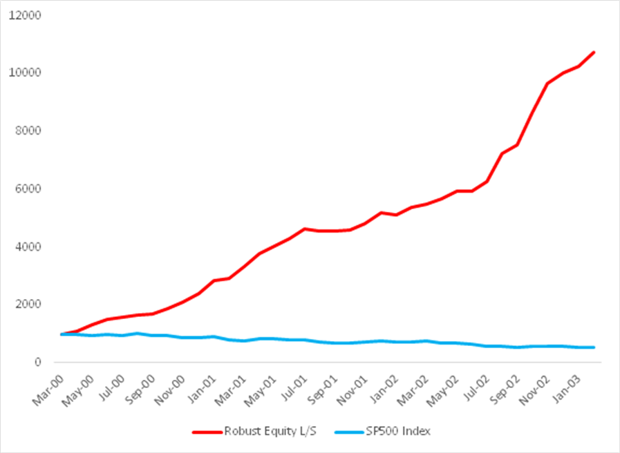
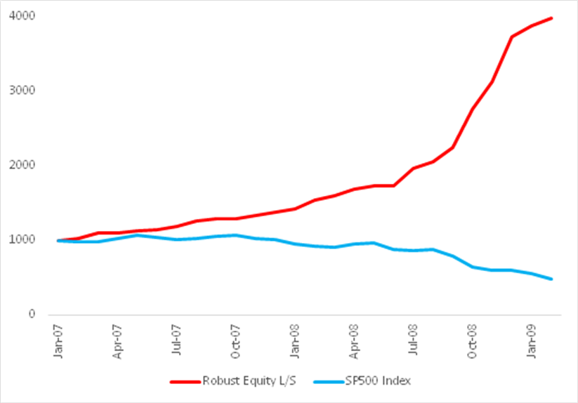
Let’s take a look at how this works out for our sample universe of twelve stocks. I will begin by focusing on the results from the two critical periods from March 2000 to Feb 2003 and from Jan 2007 to Feb 2009.
Fig. 7: Robust Equity Long/Short vs. S&P 500 index, Mar 2000-Feb 2003
Source: Yahoo Finance, 2014
Fig. 8: Robust Equity Long/Short vs. S&P 500 index, Jan 2007-Feb 2009
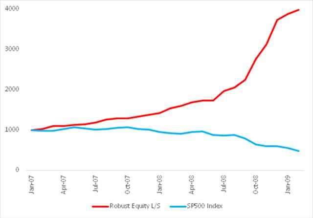
Source: Yahoo Finance, 2014
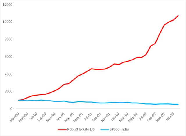
As might be imagined, given its performance during these critical periods, the overall performance of the robust portfolio dominates the market portfolio over the entire period from 1990:
Fig. 9: Robust Equity Long/Short vs. S&P 500 index, Aug 1990-Jun 2014
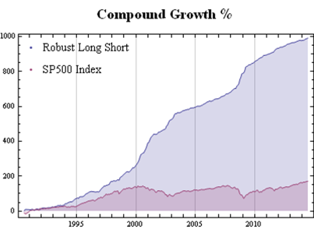
Source: Yahoo Finance, 2014
It is worth pointing out that even during benign market conditions, such as those prevailing from, say, the end of 2012, the robust portfolio outperforms the market portfolio on a risk-adjusted basis: while the returns are comparable for both, around 36% in total, the annual volatility of the robust portfolio is only 4.8%, compared to 8.4% for the S&P 500 index.
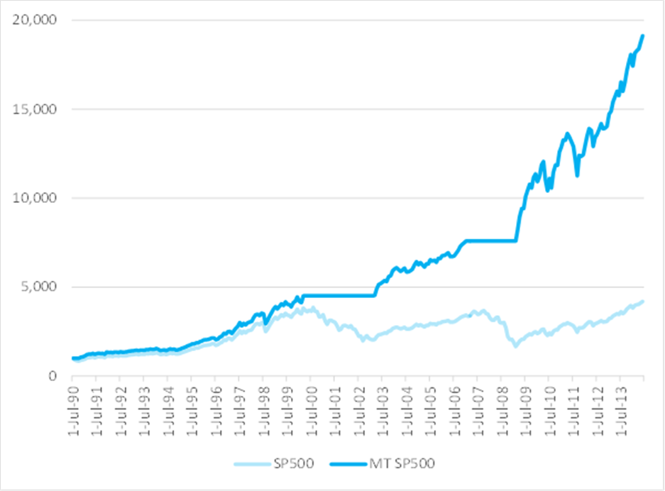
A significant benefit to the robust portfolio derives from the much lower and more stable average correlation between its constituent strategies, compared to the average correlation between the individual equities, which we considered before. As can be seen from Fig. 10, average correlation levels remained under 10% for the robust portfolio, compared to around 25% for the mean-variance optimal portfolio until 2008, rising only to a maximum value of around 15% in 2009. Thereafter, average correlation levels have drifted consistently in the downward direction, and are now very close to zero. Overall, average correlations are much more stable for the constituents in the robust portfolio than for those in the traditional portfolio: annual volatility at 12.2% is less than one-third of the annual volatility of the latter, 38.1%.
Fig. 10: Average Correlations Robust Equity Long/Short vs. S&P 500 index, Aug 1990-Jun 2014
Source: Yahoo Finance, 2014
The much lower average correlation levels mean that it is possible to construct fully diversified portfolios in the robust portfolio framework with fewer assets than in the traditional MPT framework. Put another way, a robust portfolio with a small number of assets will typically produce higher returns with lower volatility than a traditional, optimal portfolio (in the MPT sense) constructed using the same underlying assets.
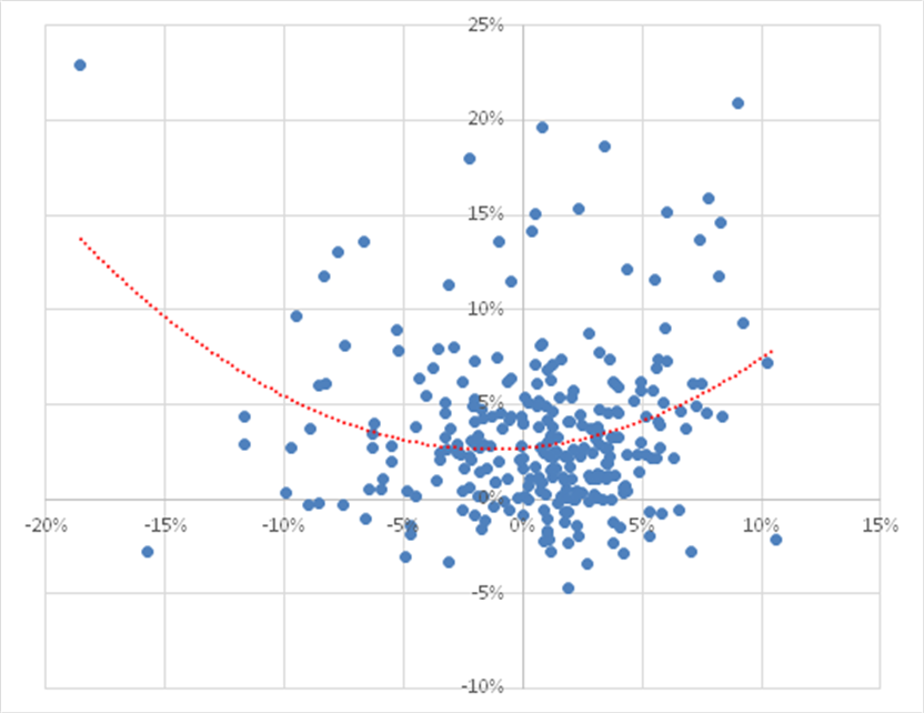
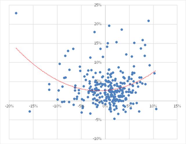
In terms of correlation of the portfolio itself, we find that over the period from Aug 1990 to June 2014, the robust portfolio exhibits close to zero net correlation with the market. However, the summary result disguises yet another important advantage of the robust portfolio. From the scatterplot shown in Fig. 11, we can see that, in fact, the robust portfolio has a tendency to adjust its correlation according to market conditions. When the market is moving positively, the robust portfolio tends to have a positive correlation, while during periods when the market is in decline, the robust portfolio tends to have a negative correlation.
Fig. 11: Correlation between Robust Equity Long/Short vs. S&P 500 index, Aug 1990-Jun 2014
Source: Yahoo Finance, 2014
Optimal Robust Portfolios
The robust portfolio referenced in our discussion hitherto is a naïve portfolio with equal dollar allocations to each individual equity strategy. What happens if we apply MPT to the equity strategy constituents and construct an “optimal” (in the mean-variance sense) robust portfolio?
The results from this procedure are summarized in Fig. 12, which shows the evolution of the efficient frontier, traversed by the risk/return path of the optimal robust portfolio. Both show considerable variability. In fact, however, both the frontier and optimal portfolio are far more stable than their equivalents for the traditional MPT strategy.
Fig. 12: Time Evolution of the Efficient Frontier and Optimal Robust Portfolio
Source: MathWorks Inc.
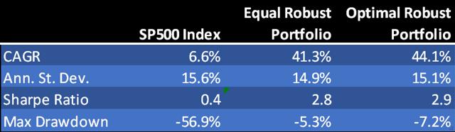
Fig. 13 compares the performance of the naïve robust portfolio and optimal robust portfolio. The optimal portfolio does demonstrate a small, material improvement in risk-adjusted returns, but at the cost of an increase in the maximum drawdown. It is an open question as to whether the modest improvement in performance is sufficient to justify the additional portfolio turnover and commensurate trading cost and operational risk. The incremental benefits are relatively minor, because the equally weighted portfolio is already well-diversified due to the low average correlation in its constituent strategies.
Fig. 13: Naïve vs. Optimal Robust Portfolio Performance Aug 1990-Jun 2014
Source: Yahoo Finance, 2014
Conclusion
The limitations of MPT in terms of its underlying assumptions and implementation challenges limits its usefulness as a practical tool for investors looking to construct equity portfolios that will enable them to achieve their investment objectives. Rather than seeking to optimize risk-adjusted returns in the traditional way, investors may be better served by identifying important characteristics of strategy robustness and using these to create strategies for individual equities that perform robustly across a wide range of market conditions. By constructing portfolios composed of such strategies, rather than using the underlying equities, investors may achieve higher, more stable returns under a broad range of market conditions, including periods of high volatility or market drawdown.
1 Optimal Versus Naive Diversification: How Inefficient is the 1/N Portfolio Strategy?, Victor DeMiguel, Lorenzo Garlappi and Raman Uppal, The Review of Financial Studies, Vol. 22, Issue 5, 2007.


 Despite the radically different programming philosophy, my experience of working with ADL has been delightfully easy and strategies that would typically take many months of coding in C++ have been up and running in a matter of days or weeks. An extract of one such strategy, a high frequency scalping trade in the E-Mini S&P 500 futures, is shown in the graphic above. The interface and visual language is so intuitive to a trading system developer that even someone who has never seen ADL before can quickly grasp at least some of what it happening in the code.
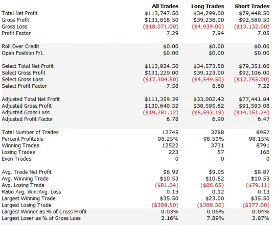 So far so good. But a 100% fill rate is clearly unrealistic. Let’s look at a pessimistic scenario: what if we got filled on orders only when the limit price was exceeded? (For those familiar with the jargon, we are assuming a high level of flow toxicity) The outcome is rather different:
 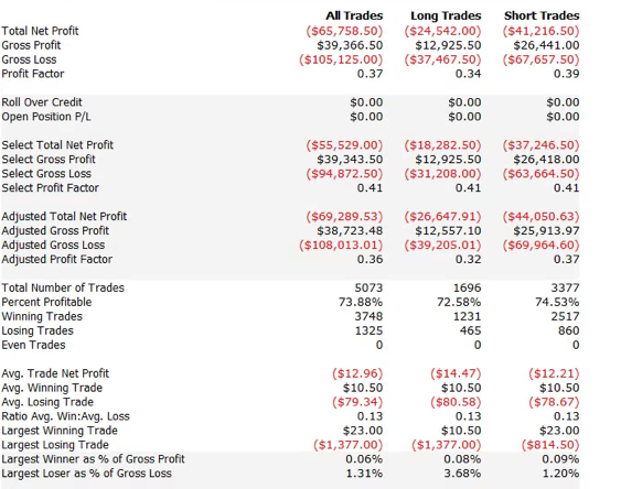 Neither scenario is particularly realistic, but the outcome is much more likely to be closer to the second scenario rather than the first if we our execution speed is slow, or if we are using a retail platform such as Interactive Brokers or Tradestation, with long latency wait times. The reason is simple: our orders will always arrive late and join the limit order book at the back of the queue. In most cases the orders ahead of ours will exhaust demand at the specified limit price and the market will trade away without filling our order. At other times the market will fill our order whenever there is a large flow against us (i.e. a surge of sell orders into our limit buy), i.e. when there is significant toxic flow. The proposition is that, using ADL and the its high-speed trading infrastructure, we can hope to avoid the latter outcome. While we will never come close to achieving a 100% fill rate, we may come close enough to offset the inevitable losses from toxic flow and produce a decent return. Whether ADL is capable of fulfilling that potential remains to be seen.