
The Reciprocal Fibonacci Constant
DataScience| Handling Big Data

Handling Large Files in CSV format with NumPy and Pandas
One of the major challenges that users face when trying to do data science is how to handle big data. Leaving aside the important topic of database connectivity/functionality and the handling of data too large to fit in memory, my concern here is with the issue of how to handle large data files, which are often in csv format, but which are not too large to fit into available memory.
It is well known that, due to their generality, Mathematica’s Import and Export functions are horribly slow when handling large csv files. For example, writing out a list of 10 million 64-bit reals takes almost 5 minutes:

and reading is also unacceptably slow:

Performance results like these create the impression that Mathematica is suitable for handling only “toy” problems, rather than the kind of large and complex data challenges faced by data scientists in the real world.
Sure, you can speed this up with ReadLine, but not by much, after doing all the string processing. And while the mx binary file format speeds up data handling enormously, it doesn’t address the issue of how to get the data into the requisite file format, other than via the WL DumpSave function – in other words, the data already has to be in a Mathematica notebook in order to write an mx file.
With purely numerical data once way to address this by using non-proprietary binary file formats. For example, in Python we create a NumPy array and use the tofile() method to output the data in real64 binary format, in less then 2 seconds:

Then in Mathematica the read process is equally fast when processing a file of numerical data in binary format, around 50x faster than the time taken to process the same file in csv format:

The procedure is just as fast in the reverse direction, with binary data exports from Mathematica taking a fraction of the time required to process the same data in csv format (around 200x faster!):

And the data is extremely fast read back in Python using the numpy fromfile method:

This procedure is robust enough to accommodate missing data. For instance, let’s replace some of the values in our data array with np.nan values and export the file once again in binary format:

Reading the binary file into Mathematica, we find no reduction in speed, as the np.nan values are stored as decimals, which are replaced by the value Indeterminate in the imported Mathematica array:

So, for purely numerical data we have a fast and reliable procedure for transferring data between Python, R and Mathematica using binary format. This means that we can load very large csv files in Python, do some pre-processing in pandas and export the massaged data in binary format for further analysis in Mathematica, if required.
More Complex Data Structures: the HDF5 Format
A major step in the right direction has been achieved through the significant effort that WR has put into implementing the HDF5 binary file format standard in the Wolfram Language. This serves two purposes: firstly, it can speed up the storage and retrieval of large datasets, by orders of magnitudes (depending on the data type); secondly, unlike Wolfram’s proprietary mx file format, HDF5 is an open source format that can store large, complex & hierarchical datasets that are accessible via Python, R and MatLab, as well as other languages/platforms, including Mathematica. So, working with the same dataset as before, but using HDF5 format, we get an speed-up of around 500x on the file write and around 270x on the file read:

Another major benefit of working in binary format is the enormous saving in disk storage, compared to csv:

So it becomes feasible to envisage a workflow in which some pre-processing of a very large dataset in csv format takes place initially in e.g. Python Pandas, the results of which are exported to a HDF5 or binary format file for further processing in Mathematica.
This advance does a great deal to address some of the major concerns about using Mathematica for large data science projects. And I am not sure that users are necessarily aware of its significance, given all the hoopla over more glamorous features that tend to get all the attention in new version releases.
Machine Learning Based Statistical Arbitrage

Previous Posts
I have written extensively about statistical arbitrage strategies in previous posts, for example:
Applying Machine Learning in Statistical Arbitrage
In this series of posts I want to focus on applications of machine learning in stat arb and pairs trading, including genetic algorithms, deep neural networks and reinforcement learning.
Pair Selection
Let’s begin with the subject of pairs selection, to set the scene. The way this is typically handled is by looking at historical correlations and cointegration in a large universe of pairs. But there are serious issues with this approach, as described in this post:
Instead I use a metric that I call the correlation signal, which I find to be a more reliable indicator of co-movement in the underlying asset processes. I wont delve into the details here, but you can get the gist from the following:
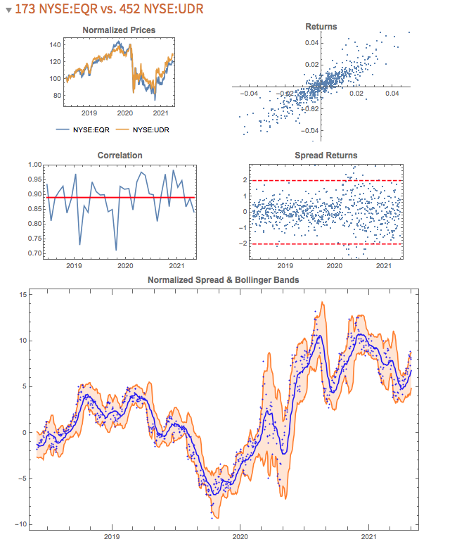
The search algorithm considers pairs in the S&P 500 membership and ranks them in descending order of correlation information. Pairs with the highest values (typically of the order of 100, or greater) tend to be variants of the same underlying stock, such as GOOG vs GOOGL, which is an indication that the metric “works” (albeit that such pairs offer few opportunities at low frequency). The pair we are considering here has a correlation signal value of around 14, which is also very high indeed.
Trading Strategy Development
We begin by collecting five years of returns series for the two stocks:
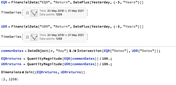
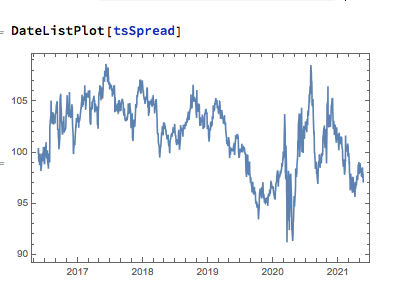
The first approach we’ll consider is the unadjusted spread, being the difference in returns between the two series, from which we crate a normalized spread “price”, as follows.
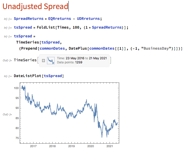
This methodology is frowned upon as the resultant spread is unlikely to be stationary, as you can see for this example in the above chart. But it does have one major advantage in terms of implementation: the same dollar value is invested in both long and short legs of the spread, making it the most efficient approach in terms of margin utilization and capital cost – other approaches entail incurring an imbalance in the dollar value of the two legs.
But back to nonstationarity. The problem is that our spread price series looks like any other asset price process – it trends over long periods and tends to wander arbitrarily far from its starting point. This is NOT the outcome that most statistical arbitrageurs are looking to achieve. On the contrary, what they want to see is a stationary process that will tend to revert to its mean value whenever it moves too far in one direction.
Still, this doesn’t necessarily determine that this approach is without merit. Indeed, it is a very typical trading strategy amongst futures traders for example, who are often looking for just such behavior in their trend-following strategies. Their argument would be that futures spreads (which are often constructed like this) exhibit clearer, longer lasting and more durable trends than in the underlying futures contracts, with lower volatility and market risk, due to the offsetting positions in the two legs. The argument has merit, no doubt. That said, spreads of this kind can nonetheless be extremely volatile.
So how do we trade such a spread? One idea is to add machine learning into the mix and build trading systems that will seek to capitalize on long term trends. We can do that in several ways, one of which is to apply genetic programming techniques to generate potential strategies that we can backtest and evaluate. For more detail on the methodology, see:
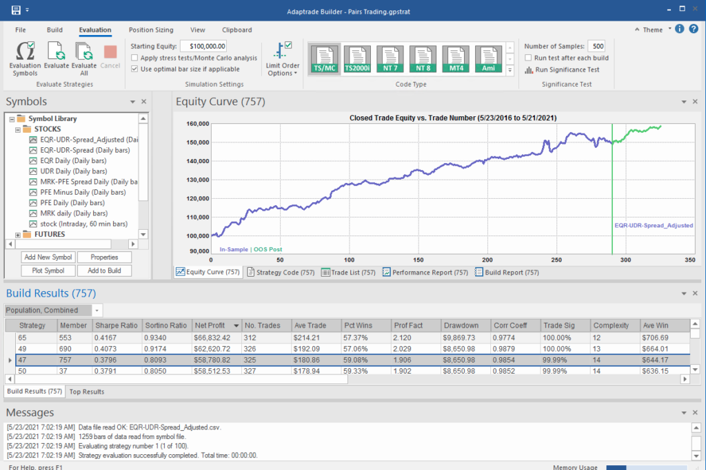
I built an entire hedge fund using this approach in the early 2000’s (when machine learning was entirely unknown to the general investing public). These days there are some excellent software applications for generating trading systems and I particularly like Mike Bryant’s Adaptrade Builder, which was used to create the strategies shown below:
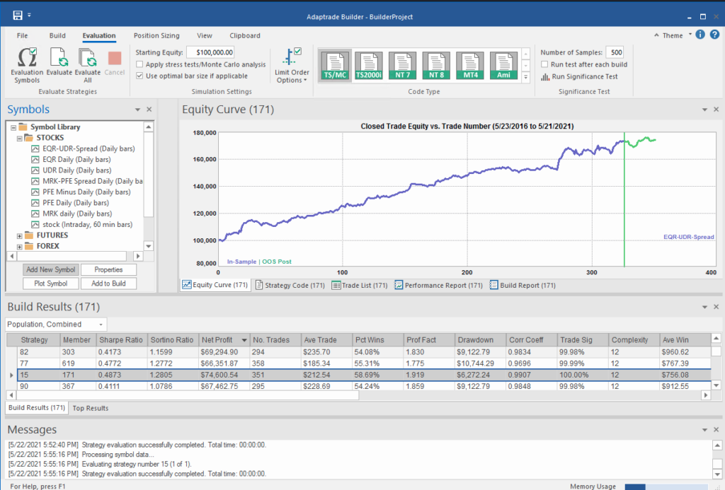
Builder has no difficulty finding strategies that produce a smooth equity curve, with decent returns, low drawdowns and acceptable Sharpe Ratios and Profit Factors – at least in backtest! Of course, there is a way to go here in terms of evaluating such strategies and proving their robustness. But it’s an excellent starting point for further R&D.
But let’s move on to consider the “standard model” for pairs trading. The way this works is that we consider a linear model of the form
Y(t) = beta * X(t) + e(t)
Where Y(t) is the returns series for stock 1, X(t) is the returns series in stock 2, e(t) is a stationary random error process and beta (is this model) is a constant that expresses the linear relationship between the two asset processes. The idea is that we can form a spread process that is stationary:
Y(t) – beta * X(t) = e(t)
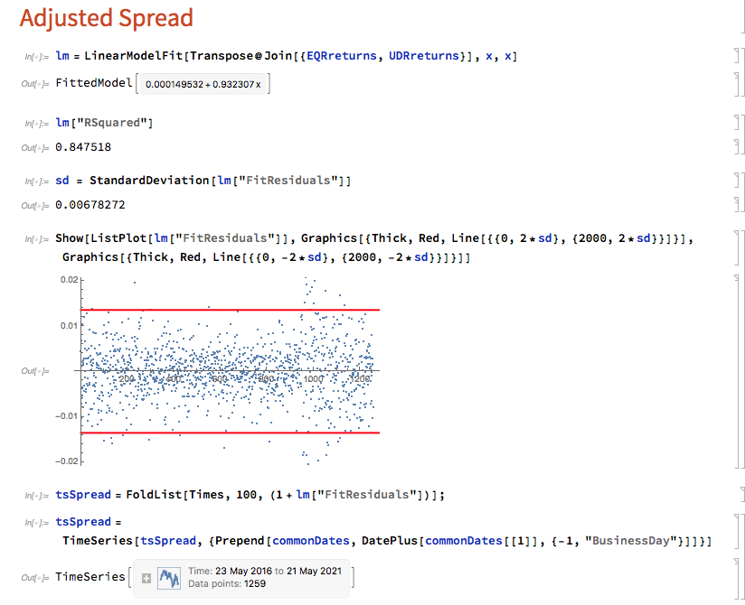
In this case we estimate beta by linear regression to be 0.93. The residual spread process has a mean very close to zero, and the spread price process remains within a range, which means that we can buy it when it gets too low, or sell it when it becomes too high, in the expectation that it will revert to the mean:
In this approach, “buying the spread” means purchasing shares to the value of, say, $1M in stock 1, and selling beta * $1M of stock 2 (around $930,000). While there is a net dollar imbalance in the dollar value of the two legs, the margin impact tends to be very small indeed, while the overall portfolio is much more stable, as we have seen.
The classical procedure is to buy the spread when the spread return falls 2 standard deviations below zero, and sell the spread when it exceeds 2 standard deviations to the upside. But that leaves a lot of unanswered questions, such as:
- After you buy the spread, when should you sell it?
- Should you use a profit target?
- Where should you set a stop-loss?
- Do you increase your position when you get repeated signals to go long (or short)?
- Should you use a single, or multiple entry/exit levels?
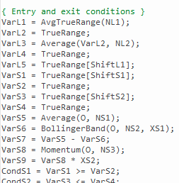
And so on – there are a lot of strategy components to consider. Once again, we’ll let genetic programming do the heavy lifting for us:
What’s interesting here is that the strategy selected by the Builder application makes use of the Bollinger Band indicator, one of the most common tools used for trading spreads, especially when stationary (although note that it prefers to use the Opening price, rather than the usual close price):
Ok so far, but in fact I cheated! I used the entire data series to estimate the beta coefficient, which is effectively feeding forward-information into our model. In reality, the data comes at us one day at a time and we are required to re-estimate the beta every day.
Let’s approximate the real-life situation by re-estimating beta, one day at a time. I am using an expanding window to do this (i.e. using the entire data series up to each day t), but is also common to use a fixed window size to give a “rolling” estimate of beta in which the latest data plays a more prominent part in the estimation. The process now looks like this:
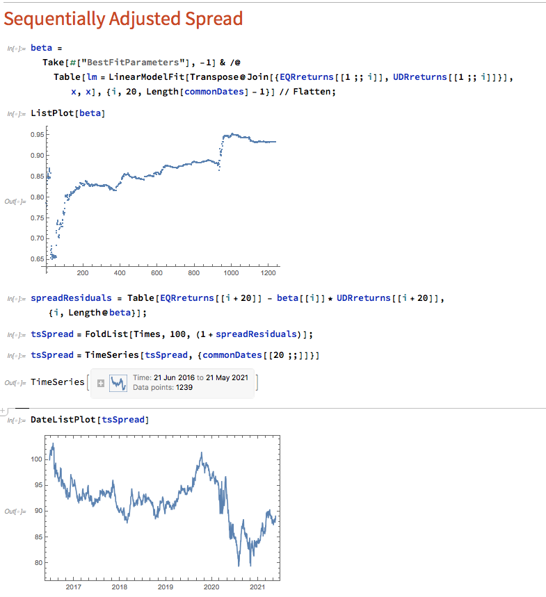
Here we use OLS to produce a revised estimate of beta on each trading day. So our model now becomes:
Y(t) = beta(t) * X(t) + e(t)
i.e. beta is now time-varying, as can be seen from the chart above.
The synthetic spread price appears to be stationary (we can test this), although perhaps not to the same degree as in the previous example, where we used the entire data series to estimate a single, constant beta. So we might anticipate that out ML algorithm would experience greater difficulty producing attractive trading models. But, not a bit of it – it turns out that we are able to produce systems that are just as high performing as before:
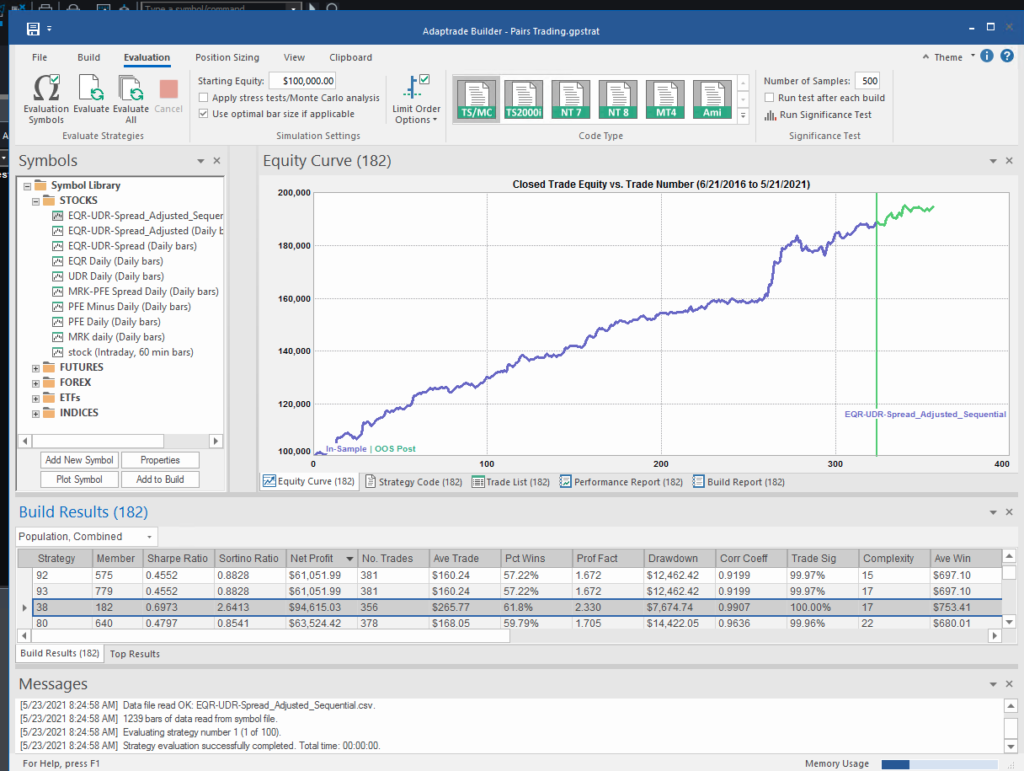
In fact this strategy has higher returns, Sharpe Ratio, Sortino Ratio and lower drawdown than many of the earlier models.
Conclusion
The purpose of this post was to show how we can combine the standard approach to statistical arbitrage, which is based on classical econometric theory, with modern machine learning algorithms, such as genetic programming. This frees us to consider a very much wider range of possible trade entry and exit strategies, beyond the rather simplistic approach adopted when pairs trading was first developed. We can deploy multiple trade entry levels and stop loss levels to manage risk, dynamically size the trade according to current market conditions and give emphasis to alternative performance characteristics such as maximum drawdown, or Sharpe or Sortino ratio, in addition to strategy profitability.
The programatic nature of the strategies developed in the way also make them very amenable to optimization, Monte Carlo simulation and stress testing.
This is but one way of adding machine learning methodologies to the mix. In a series of follow-up posts I will be looking at the role that other machine learning techniques – such as deep learning and reinforcement learning – can play in improving the performance characteristics of the classical statistical arbitrage strategy.
A Study in Gold

I want to take a look at a trading strategy in the GDX Gold ETF that has attracted quite a lot of attention, stemming from Jay Kaeppel’s article: The Greatest Gold Stock System You’ll Probably Never Use .
The essence of the approach is that GDX has reliably tended to trade off during the day session, after making gains in the overnight session. One possible explanation for the phenomenon is offer by Adrian Douglas in his article Gold Market is not “Fixed”, it’s Rigged in which he takes issue with the London Fixing mechanism used to set the daily price of gold
In any event there has been a long-term opportunity to exploit what appears to be a market inefficiency using an extremely simple trading rule, as described by Oddmund Grotte (see http://www.quantifiedstrategies.com/the-greatest-gold-stock-system-you-should-trade/):
1) If GDX rises from the open to the close more than 0.1%, buy on the close and exit on the opening next day.
2) If GDX rises from the open to the close more than 0.1% the day before, sell short on the opening and exit on the close (you have to both sell your position from number 1 but also short some more).

Unfortunately this simple strategy has recently begun to fail, producing (substantial) negative returns since June 2013. So I have been experimenting with a number of closely-related strategies and have created a simple Excel workbook to evaluate them. First, a little notation:
RCO = Return from prior close to market open
ROC = return from open to close
RCC = Return from close to close
I also use the suffix “m1” to denote the prior period’s return. So, for example, ROCm1 is yesterday’s return, measured from open to close. And I use the slash symbol “/” to denote dependency. So, for instance, RCO/ROCm1 means the return from today’s open to close, given the return from open to close yesterday.
In the accompanying workbook I look at several possible, closely related trading rules, and evaluate their performance over time. The basic daily data spans the period from May 2006 to July 2013 and in shown in columns A-H of the workbook. Columns I-K show the daily RCO, ROC and RCC returns. The returns for three different strategies are shown in columns L, N and P, and the cumulative returns for each are shown in columns M, N and Q, respectively.
The trading rules for each of the strategies are as follows:
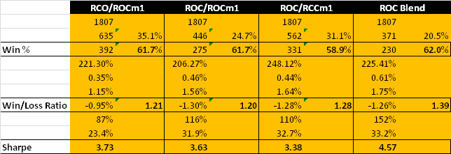
COL L: RCO/ROCm1>0.5%. Which means: buy GDX at the close if the intra-day return from open to close exceeds 0.5%, and hold overnight until the following morning.
COL N: ROC/ROCm1>1%. Which means: sell GDX at today’s open if the intra-day return from open to close on the preceding day exceeds 1% and buy at today’s close.
COL P: ROC/RCCm1>1%. Which means: sell GDX at today’s open if the return from close to close on the preceding day exceeds 1% and buy at today’s close.
COL R shows returns from a blended strategy which combines the returns from the strategies in columns N and P on Mondays, Tuesdays and Thursdays only (i.e. assuming no trading on Wednesdays or Fridays). The cumulative returns from this hybrid strategy are shown in column S.
We can now present the results from the four strategies, over the 7 year period from May 2006 to July 2013, as shown in the chart and table below. On their face, the results are impressive: all four strategies have Sharpe ratios in excess of 3, with the blended strategy having a Sharpe of 4.57, while the daily win rates average around 60%.

How well do these strategies hold up over time? You can monitor their performance as you move through time by clicking on the scrollbar control in COL U of the workbook. As you do so, the start date of the strategies is rolled forward, and the table of performance results is updated to include results from the new start date, ignoring any prior data.
As you can see, all of the strategies continue to perform well into the latter part of 2010. At that point, the performance of the first strategy begins to decline precipitously, although the remaining three strategies continue to do well. By mid-2012, the first strategy is showing negative performance, while the Sharpe ratios of the remaining strategies begin to decline. As we reach the end of Q1, 2013, only the Sharpe ratio of the ROC/RCCm1 strategy remains above 2 for the period Apr 2013 to July 2013.
The conclusion appears to be that there is evidence for the possibility of generating abnormal returns in GDX lasting well into the current decade. However these have declined considerably in recent years, to a point where the effects are likely no longer important.
Strategy Backtesting in Mathematica
This is a snippet from a strategy backtesting system that I am currently building in Mathematica.
One of the challenges when building systems in WL is to avoid looping wherever possible. This can usually be accomplished with some thought, and the efficiency gains can be significant. But it can be challenging to get one’s head around the appropriate construct using functions like FoldList, etc, especially as there are often edge cases to be taken into consideration.
A case in point is the issue of calculating the profit and loss from individual trades in a trading strategy. The starting point is to come up with a FoldList compatible function that does the necessary calculations:
CalculateRealizedTradePL[{totalQty_, totalValue_, avgPrice_, PL_,
totalPL_}, {qprice_, qty_}] :=
Module[{newTotalPL = totalPL, price = QuantityMagnitude[qprice],
newTotalQty, tradeValue, newavgPrice, newTotalValue, newPL},
newTotalQty = totalQty + qty;
tradeValue =
If[Sign[qty] == Sign[totalQty] || avgPrice == 0, priceqty, If[Sign[totalQty + qty] == Sign[totalQty], avgPriceqty,
price(totalQty + qty)]]; newTotalValue = If[Sign[totalQty] == Sign[newTotalQty], totalValue + tradeValue, newTotalQtyprice];
newavgPrice =
If[Sign[totalQty + qty] ==
Sign[totalQty], (totalQtyavgPrice + tradeValue)/newTotalQty, price]; newPL = If[(Sign[qty] == Sign[totalQty] ) || totalQty == 0, 0, qty(avgPrice - price)];
newTotalPL = newTotalPL + newPL;
{newTotalQty, newTotalValue, newavgPrice, newPL, newTotalPL}]
Trade P&L is calculated on an average cost basis, as opposed to FIFO or LIFO.
Note that the functions handle both regular long-only trading strategies and short-sale strategies, in which (in the case of equities), we have to borrow the underlying stock to sell it short. Also, the pointValue argument enables us to apply the functions to trades in instruments such as futures for which, unlike stocks, the value of a 1 point move is typically larger than 1(e.g.50 for the ES S&P 500 mini futures contract).
We then apply the function in two flavors, to accommodate both standard numerical arrays and timeseries (associations would be another good alternative):
CalculateRealizedPLFromTrades[tradeList_?ArrayQ, pointValue_ : 1] :=
Module[{tradePL =
Rest@FoldList[CalculateRealizedTradePL, {0, 0, 0, 0, 0},
tradeList]},
tradePL[[All, 4 ;; 5]] = tradePL[[All, 4 ;; 5]]pointValue; tradePL] CalculateRealizedPLFromTrades[tsTradeList_, pointValue_ : 1] := Module[{tsTradePL = Rest@FoldList[CalculateRealizedTradePL, {0, 0, 0, 0, 0}, QuantityMagnitude@tsTradeList["Values"]]}, tsTradePL[[All, 4 ;; 5]] = tsTradePL[[All, 4 ;; 5]]pointValue;
tsTradePL[[All, 2 ;;]] =
Quantity[tsTradePL[[All, 2 ;;]], "US Dollars"];
tsTradePL =
TimeSeries[
Transpose@
Join[Transpose@tsTradeList["Values"], Transpose@tsTradePL],
tsTradeList["DateList"]]]
These functions run around 10x faster that the equivalent functions that use Do loops (without parallelization or compilation, admittedly).
Let’s see how they work with an example:
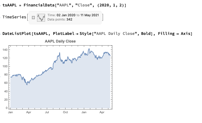
Trade Simulation
Next, we’ll generate a series of random trades using the AAPL time series, as follows (we also take the opportunity to convert the list of trades into a time series, tsTrades):
trades = Transpose@
Join[Transpose[
tsAAPL["DatePath"][[
Sort@RandomSample[Range[tsAAPL["PathLength"]],
20]]]], {RandomChoice[{-100, 100}, 20]}];
trades // TableForm
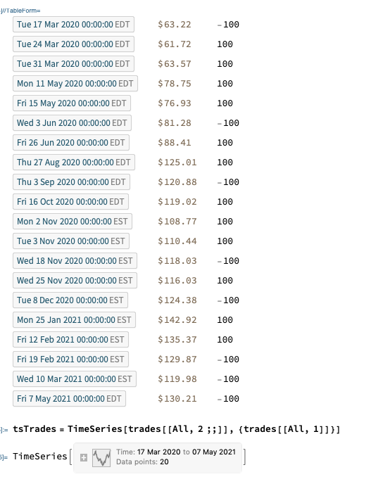
Trade P&L Calculation
We are now ready to apply our Trade P&L calculation function, first to the list of trades in array form:
TableForm[
Flatten[#] & /@
Partition[
Riffle[trades,
CalculateRealizedPLFromTrades[trades[[All, 2 ;; 3]]]], 2],
TableHeadings -> {{}, {"Date", "Price", "Quantity", "Total Qty",
"Position Value", "Average Price", "P&L", "Total PL"}}]
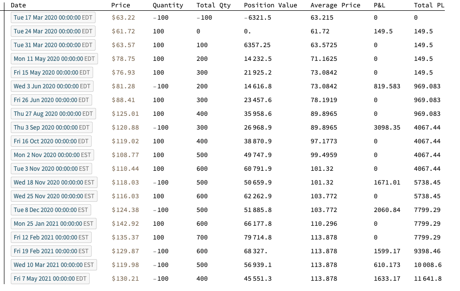
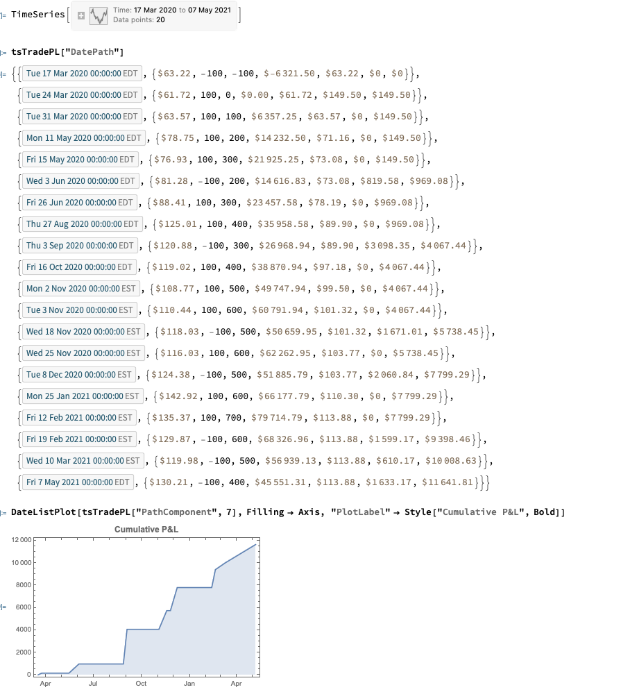
The timeseries version of the function provides the output as a timeseries object in Quantity[“US Dollars”] format and, of course, can be plotted immediately with DateListPlot (it is also convenient for other reasons, as the complete backtest system is built around timeseries objects):
tsTradePL = CalculateRealizedPLFromTrades[tsTrades]

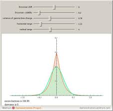
Implied Volatility in Merton’s Jump Diffusion Model

The “implied volatility” corresponding to an option price is the value of the volatility parameter for which the Black-Scholes model gives the same price. A well-known phenomenon in market option prices is the “volatility smile”, in which the implied volatility increases for strike values away from the spot price. The jump diffusion model is a generalization of Black\[Dash]Scholes in which the stock price has randomly occurring jumps in addition to the random walk behavior. One of the interesting properties of this model is that it displays the volatility smile effect. In this Demonstration, we explore the Black-Scholes implied volatility of option prices (equal for both put and call options) in the jump diffusion model. The implied volatility is modeled as a function of the ratio of option strike price to spot price.
Option Prices in the Variance Gamma Model
Measuring Toxic Flow for Trading & Risk Management

A common theme of microstructure modeling is that trade flow is often predictive of market direction. One concept in particular that has gained traction is flow toxicity, i.e. flow where resting orders tend to be filled more quickly than expected, while aggressive orders rarely get filled at all, due to the participation of informed traders trading against uninformed traders. The fundamental insight from microstructure research is that the order arrival process is informative of subsequent price moves in general and toxic flow in particular. This is turn has led researchers to try to measure the probability of informed trading (PIN). One recent attempt to model flow toxicity, the Volume-Synchronized Probability of Informed Trading (VPIN)metric, seeks to estimate PIN based on volume imbalance and trade intensity. A major advantage of this approach is that it does not require the estimation of unobservable parameters and, additionally, updating VPIN in trade time rather than clock time improves its predictive power. VPIN has potential applications both in high frequency trading strategies, but also in risk management, since highly toxic flow is likely to lead to the withdrawal of liquidity providers, setting up the conditions for a flash-crash” type of market breakdown.
The procedure for estimating VPIN is as follows. We begin by grouping sequential trades into equal volume buckets of size V. If the last trade needed to complete a bucket was for a size greater than needed, the excess size is given to the next bucket. Then we classify trades within each bucket into two volume groups: Buys (V(t)B) and Sells (V(t)S), with V = V(t)B + V(t)S
The Volume-Synchronized Probability of Informed Trading is then derived as:

Typically one might choose to estimate VPIN using a moving average over n buckets, with n being in the range of 50 to 100.
Another related statistic of interest is the single-period signed VPIN. This will take a value of between -1 and =1, depending on the proportion of buying to selling during a single period t.

Fig 1. Single-Period Signed VPIN for the ES Futures Contract
It turns out that quote revisions condition strongly on the signed VPIN. For example, in tests of the ES futures contract, we found that the change in the midprice from one volume bucket the next was highly correlated to the prior bucket’s signed VPIN, with a coefficient of 0.5. In other words, market participants offering liquidity will adjust their quotes in a way that directly reflects the direction and intensity of toxic flow, which is perhaps hardly surprising.
Of greater interest is the finding that there is a small but statistically significant dependency of price changes, as measured by first buy (sell) trade price to last sell (buy) trade price, on the prior period’s signed VPIN. The correlation is positive, meaning that strongly toxic flow in one direction has a tendency to push prices in the same direction during the subsequent period. Moreover, the single period signed VPIN turns out to be somewhat predictable, since its autocorrelations are statistically significant at two or more lags. A simple linear auto-regression ARMMA(2,1) model produces an R-square of around 7%, which is small, but statistically significant.
A more useful model, however , can be constructed by introducing the idea of Markov states and allowing the regression model to assume different parameter values (and error variances) in each state. In the Markov-state framework, the system transitions from one state to another with conditional probabilities that are estimated in the model.
An example of such a model for the signed VPIN in ES is shown below. Note that the model R-square is over 27%, around 4x larger than for a standard linear ARMA model.
We can describe the regime-switching model in the following terms. In the regime 1 state the model has two significant autoregressive terms and one significant moving average term (ARMA(2,1)). The AR1 term is large and positive, suggesting that trends in VPIN tend to be reinforced from one period to the next. In other words, this is a momentum state. In the regime 2 state the AR2 term is not significant and the AR1 term is large and negative, suggesting that changes in VPIN in one period tend to be reversed in the following period, i.e. this is a mean-reversion state.
The state transition probabilities indicate that the system is in mean-reversion mode for the majority of the time, approximately around 2 periods out of 3. During these periods, excessive flow in one direction during one period tends to be corrected in the
ensuring period. But in the less frequently occurring state 1, excess flow in one direction tends to produce even more flow in the same direction in the following period. This first state, then, may be regarded as the regime characterized by toxic flow.
Markov State Regime-Switching Model
Markov Transition Probabilities
P(.|1) P(.|2)
P(1|.) 0.54916 0.27782
P(2|.) 0.45084 0.7221
Regime 1:
AR1 1.35502 0.02657 50.998 0
AR2 -0.33687 0.02354 -14.311 0
MA1 0.83662 0.01679 49.828 0
Error Variance^(1/2) 0.36294 0.0058
Regime 2:
AR1 -0.68268 0.08479 -8.051 0
AR2 0.00548 0.01854 0.296 0.767
MA1 -0.70513 0.08436 -8.359 0
Error Variance^(1/2) 0.42281 0.0016
Log Likelihood = -33390.6
Schwarz Criterion = -33445.7
Hannan-Quinn Criterion = -33414.6
Akaike Criterion = -33400.6
Sum of Squares = 8955.38
R-Squared = 0.2753
R-Bar-Squared = 0.2752
Residual SD = 0.3847
Residual Skewness = -0.0194
Residual Kurtosis = 2.5332
Jarque-Bera Test = 553.472 {0}
Box-Pierce (residuals): Q(9) = 13.9395 {0.124}
Box-Pierce (squared residuals): Q(12) = 743.161 {0}
A Simple Trading Strategy
One way to try to monetize the predictability of the VPIN model is to use the forecasts to take directional positions in the ES
contract. In this simple simulation we assume that we enter a long (short) position at the first buy (sell) price if the forecast VPIN exceeds some threshold value 0.1 (-0.1). The simulation assumes that we exit the position at the end of the current volume bucket, at the last sell (buy) trade price in the bucket.
This simple strategy made 1024 trades over a 5-day period from 8/8 to 8/14, 90% of which were profitable, for a total of $7,675 – i.e. around ½ tick per trade.
The simulation is, of course, unrealistically simplistic, but it does give an indication of the prospects for more realistic version of the strategy in which, for example, we might rest an order on one side of the book, depending on our VPIN forecast.

Figure 2 – Cumulative Trade PL
References
Easley, D., Lopez de Prado, M., O’Hara, M., Flow Toxicity and Volatility in a High frequency World, Johnson School Research paper Series # 09-2011, 2011
Easley, D. and M. O‟Hara (1987), “Price, Trade Size, and Information in Securities Markets”, Journal of Financial Economics, 19.
Easley, D. and M. O‟Hara (1992a), “Adverse Selection and Large Trade Volume: The Implications for Market Efficiency”,
Journal of Financial and Quantitative Analysis, 27(2), June, 185-208.
Easley, D. and M. O‟Hara (1992b), “Time and the process of security price adjustment”, Journal of Finance, 47, 576-605.
Generalized Regression
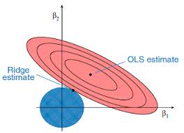
Linear regression is one of the most useful applications in the financial engineer’s tool-kit, but it suffers from a rather restrictive set of assumptions that limit its applicability in areas of research that are characterized by their focus on highly non-linear or correlated variables. The latter problem, referred to as colinearity (or multicolinearity) arises very frequently in financial research, because asset processes are often somewhat (or even highly) correlated. In a colinear system, one can test for the overall significant of the regression relationship, but one is unable to distinguish which of the explanatory variables is individually significant. Furthermore, the estimates of the model parameters, the weights applied to each explanatory variable, tend to be biased.
Over time, many attempts have been made to address this issue, one well-known example being ridge regression. More recent attempts include lasso, elastic net and what I term generalized regression, which appear to offer significant advantages vs traditional regression techniques in situations where the variables are correlated.
In this note, I examine a variety of these techniques and attempt to illustrate and compare their effectiveness.

The Mathematica notebook is also available here.