Stock Price Range Forecasts
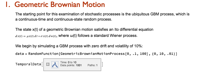
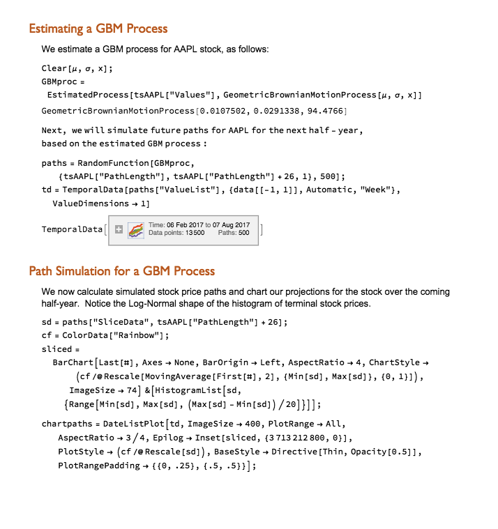
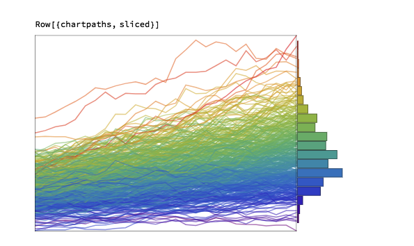
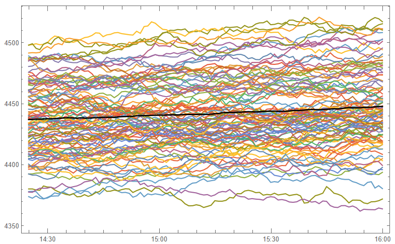
Range forecasts are produced by estimating the parameters of a Geometric Brownian Motion process from historical data and using the model to project a large number of sample paths for the stock price over the coming month and year.
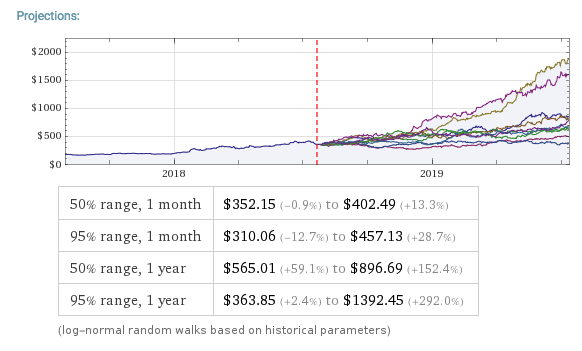
For example, this is a range forecast for Netflix, Inc. (NFLX) as at 7/27/2018 when the price of the stock stood at $355.21:

As you can see, the great majority of the simulated price paths trend upwards. This is typical for most stocks on account of their upward drift, a tendency to move higher over time. The statistical table below the chart tells you that in 50% of cases the ending stock price 1 month from the date of forecast was in the range $352.15 to $402.49. Similarly, around 50% of the time the price of the stock in one year’s time were found to be in the range $565.01 to $896.69. Notice that the end points of the one-year range far exceed the end points of the one-month range forecast – again this is a feature of the upward drift in stocks.
If you want much greater certainty about the outcome, you should look at the 95% ranges. So, for NFLX, the one month 95% range was projected to be $310.06 to $457.13. Here, only 1 in 20 of the simulated price paths produced one month forecasts that were higher than $457.13, or lower than $310.06.
Notice that the spread of the one month and one year 95% ranges is much larger than of the corresponding 50% ranges. This demonstrates the fundamental tradeoff between “accuracy” (the spread of the range) and “certainty”, (the probability of the outcome being with the projected range). If you want greater certainty of the outcome, you have to allow for a broader span of possibilities, i.e. a wider range.

Uses of Range Forecasts
Most stock analysts tend to produce single price “targets”, rather than a range – these are known as “point forecasts” by econometricians. So what’s the thinking behind range forecasts?
Range forecasts are arguably more useful than simple point forecasts. Point forecasts make no guarantee as to the likelihood of the projected price – the only thing we know for sure about such forecasts is that they will be wrong! Is the forecast target price optimistic or pessimistic? We have no way to tell.
With range forecasts the situation is very different. We can talk about the likelihood of a stock being within a specified range at a certain point in time. If we want to provide a pessimistic forecast for the price in NFLX in one month’s time, for example, we could quote the value $352.15, the lower end of the 50% range forecast. If we wanted to provide a very pessimistic forecast, one that is very likely to be exceeded, we could quote the bottom of the 95% range: $310.06.
The range also tells us about the future growth prospects for the firm. So, for example, with NFLX, based on past performance, it is highly likely that the stock price will grow at a rate of more than 2.4% and, optimistically, might increase by almost 3x in the coming year (see the growth rates calculated for the 95% range values).
One specific use of range forecasts is in options trading. If a trader is bullish on NFLX, instead of buying the stock, he might instead choose to sell one-month put options with a strike price below $352 (the lower end of the 50% one-month range). If the trader wanted to be more conservative, he might look for put options struck at around $310, the bottom of the 95% range. A more complex strategy might be to buy calls struck near the top of the 50% range, and sell more calls struck near the top of the 95% range (the theory being that the stock is quite likely to exceed the top of the 50% one-month range, but much less likely to reach the high end of the 95% range).
Limitations of Range Forecasts
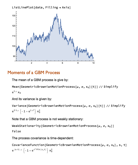
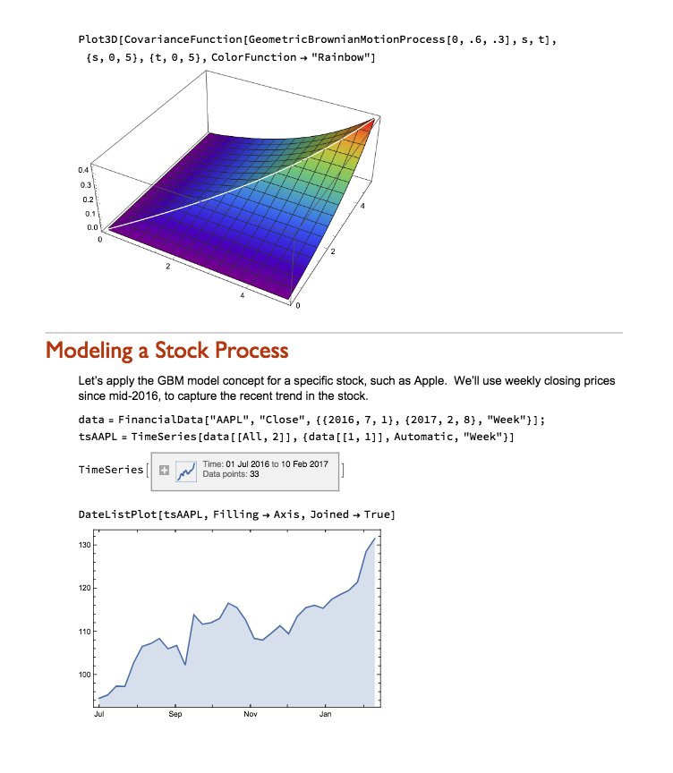
Range forecasts are produced by using historical data to estimate the parameters of a particular type of mathematical model, known as a Geometric Brownian Motion process. For those who are interested in the mechanics of how the forecasts are produced, I have summarized the relevant background theory below.
While there are grounds for challenging the use of such models in this context, it has to be acknowledged that the GBM process is one of the most successful mathematical models in finance today. The problem lies not so much in the model, as in one of the key assumptions underpinning the approach: specifically, that the characteristics of the stock process will remain as they are today (and as they have been in the historical past). This assumption is manifestly untenable when applied to many stocks: a company that was a high-growth $100M start-up is unlikely to demonstrate the same rate of growth ten years later, as a $10Bn enterprise. A company like Amazon that started out as an online book seller has fundamentally different characteristics today, as an online retail empire. In such cases, forecasts about the future stock price – whether point or range forecasts – based on outdated historical informations are likely to be wrong, sometimes wildly so.
Having said that, there are a great many companies that have evolved to a point of relative stability over a period of perhaps several decades: for example, a company like Caterpillar Inc. (CAT). In such cases the parameters of the GBM process underpinning the stock price are unlikely to fluctuate widely in the short term, so range forecasts are consequently more likely to be useful.
Another factor to consider are quarterly earnings reports, which can influence stock prices considerably in the short term, and corporate actions (mergers, takeovers, etc) that can change the long term characteristics of a firm and its stock price process in a fundamental way. In these situations any forecast methodology is likely to unreliable, at least for a while, until the event has passed. It’s best to avoid taking positions based on projections from historical data at times like this.
Review of Background Theory
