In a post on LinkedIn I referred to the concept of CrashMetrics and how it can be used for portfolio protection. It’s a simple approach to the management of extreme risk that works rather well. It can be summarized as “CAPM for crashes”. Here’s how it works.
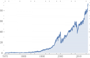
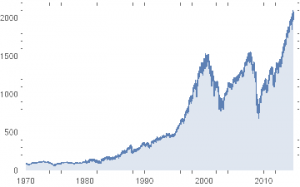
Let’s take Proctor and Gamble as our example stock. We’ll use daily data from 1970-2014 for the stock and for the S&P 500 Index, as follows:
DateListPlot[PG=TimeSeries[FinancialData[“PG”,{{1970,1,2},{2014,12,31}}]],Filling->Axis]
DateListPlot[SP500=TimeSeries[FinancialData[“^GSPC”,{{1970,1,2},{2014,12,31}}]],Filling->Axis]
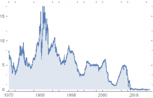
We are also going to need an estimate of the risk free rate of return. We’ll use a 30-day T-Bill rate:
DateListPlot[TBill=TimeSeries[FinancialData[“^IRX”,{{1970,1,2},{2014,12,31}}]],Filling->Axis]
CAPM Beta Estimation
Next we convert the annual Bill yields into estimates of the continuously compounded daily return and subtract these from the gross returns for PG and the S&P 500 Index, to create series of excess returns for the stock and the index.
SP500Dates=SP500[“Times”]
PGReturns=Log[PG[Drop[SP500Dates,1]]]-Log[PG[Drop[SP500Dates,-1]]];
SP500Returns=Log[Drop[SP500[“Values”],1]]-Log[Drop[SP500[“Values”],-1]];
TBillDailyRate=Log[TBill[Drop[SP500Dates,1]]]/250 /. Indeterminate->0;
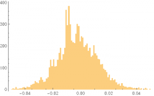
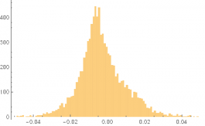
Histogram[PGXReturns=PGReturns-TBillDailyRate,{-0.05,0.05,0.001}]
Excess Returns PG 1970-2014
Excess Returns S&P 500 Index 1970-2014
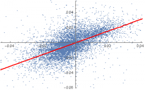
We are now ready to estimate the stock beta for PG, using a simple linear regression model of the excess returns in the stock vs. the excess returns in the S&P 500 Index:
dataset=Partition[Riffle[SP500XReturns,PGXReturns],2
CAPM = LinearModelFit[dataset,x,x]
From which we estimate the beta for PG to be around 0.78 (the slope of the regression line in the scatterplot below). That seems plausible for a large, diversified consumer goods manufacturer, which is likely to be less volatile than the broad index during normal market conditions.
Show[ListPlot[dataset],Plot[CAPM[x],{x,-0.05,0.05},PlotStyle->Red]]
The CAPM regression shows that around 40% of the variation in excess returns in PG is explained by movements in the broad market (the remainder is due to stock-specific risk factors):
CAPM[“AdjustedRSquared”] = 0.40
That’s a typically scenario with the CAPM model, which is based on some fairly simple, but rather heroic assumptions that we need not delve too deeply into here.
CrashMetrics Approach
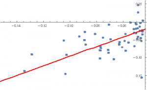
In CrashMetrics we focus exclusively in the left tail of the distribution. For the S&P 500 index the average excess return is very close to zero, while the daily standard deviation of returns is just over 1.5%. So let’s focus on down-moves that are, say, at least 3xSD, or larger. We create a reduced data set comprising days on which the index declined by at least 4.5%, and repeat the regression procedure using just those 54 days:
Dimensions[reducedDataset=Select[dataset,#[[1]] < -0.045&]{54,2}
CrashM = LinearModelFit[reducedDataset,x,x]
Show[ListPlot[reducedDataset],Plot[CrashM[x],{x,0, -0.25},PlotStyle->Red]]
Two points are especially noteworthy.
The first is that the beta for PG during major market down-moves is a lot higher than during normal markets (around 1.34 vs 0.78) and being greater than 1, indicates that during adverse conditions PG tends to exacerbate the down-turn in the broad market.
The second is that the regression R-squared is much higher (0.68) for the CrashMetrics regression model, reflecting the tendency of stocks to correlate more closely with the market index during major sell-offs. In that sense, the “crash-beta” estimate is a more reliable estimate than the regular CAPM beta.
How to Use CrashMetrics
How is this technique helpful to the portfolio manager?
To begin, you might want to estimate crash-betas for all of the stocks in your portfolio and for the portfolio as a whole, to give you a handle on how the portfolio is likely to behave under extreme stress.
You could then choose to make adjustments to the portfolio composition to reduce its crash exposure. This can be done by reducing the allocations to high crash-beta stocks in favor of low crash-beta stocks. Alternatively, you can buy tail protection using out-of-the-money put options in high-crash beta stocks. What’s interesting about this technique is that you might end up paying less for crash-protection than you might think.
Taking our PG test case as an example, this is typically seen as a less risky stock and its options are priced accordingly. Consequently, the Gamma in the options looks cheap when considering how the stock behaves during market crashes. Conversely, options in very volatile stocks (AAPL springs to mind, for example), are likely to be relatively highly priced, but may offer less protection during a crash scenario, depending on the behavior of the stock during major market declines.
