Introduction
When we launched the Equities Entity Store in Mathematica, it revolutionized how financial professionals interact with market data by bringing semantic structure, rich metadata, and analysis-ready information into a unified framework. Mathematica’s EntityStore provided an elegant way to explore equities, ETFs, indices, and factor models through a symbolic interface. However, the industry landscape has evolved—the majority of quantitative finance, data science, and machine learning now thrives in Python.
While platforms like FactSet, WRDS, and Bloomberg provide extensive financial data, quantitative researchers still spend up to 80% of their time wrangling data rather than building models. Current workflows often involve downloading CSV files, manually cleaning them in pandas, and stitching together inconsistent time series—all while attempting to avoid subtle lookahead bias that invalidates backtests.
Recognizing these challenges, we’ve reimagined the Equities Entity Store for Python, focusing first on what the Python ecosystem does best: scalable machine learning and robust data analysis.
The Python Version: What’s New
Rather than beginning with metadata-rich entity hierarchies, the Python Equities Entity Store prioritizes the intersection of high-quality data and predictive modeling capabilities. At its foundation lies a comprehensive HDF5 dataset containing over 1,400 features for 7,500 stocks, measured monthly from 1995 to 2025—creating an extensive cross-sectional dataset optimized for sophisticated ML applications.
Our lightweight, purpose-built package includes specialized modules for:
- Feature loading: Efficient extraction and manipulation of data from the HDF5 store
- Feature preprocessing: Comprehensive tools for winsorization, z-scoring, neutralization, and other essential transformations
- Label construction: Flexible creation of target variables, including 1-month forward information ratio
- Ranking models: Advanced implementations including LambdaMART and other gradient-boosted tree approaches
- Portfolio construction: Sophisticated tools for converting model outputs into actionable investment strategies
- Backtesting and evaluation: Rigorous performance assessment across multiple metrics
Guaranteed Protection Against Lookahead Bias
A critical advantage of our Python Equities Entity Store implementation is its robust safeguards against lookahead bias—a common pitfall that compromises the validity of backtests and predictive models. Modern ML preprocessing pipelines often inadvertently introduce information from the future into training data, leading to unrealistic performance expectations.
Unlike platforms such as QuantConnect, Zipline, or even custom research environments that require careful manual controls, our system integrates lookahead protection at the architectural level:
# Example: Time-aware feature standardization with strict temporal boundaries
from equityentity.features.preprocess import TimeAwareStandardizer

# This standardizer only uses data available up to each point in time
standardizer = TimeAwareStandardizer(lookback_window='60M')
zscore_features = standardizer.fit_transform(raw_features)

# Instead of the typical approach that inadvertently leaks future data:

# DON'T DO THIS: sklearn.preprocessing.StandardScaler().fit_transform(raw_features)
Multiple safeguards are integrated throughout the system:
- Time-aware preprocessing: All transformations (normalization, imputation, feature engineering) strictly respect temporal boundaries
- Point-in-time data snapshots: Features reflect only information available at the decision point
- New listing delay: Stocks are only included after a customizable delay period from their first trading date
# From our data_loader.py - IPO bias protection through months_delay

for i, symbol in enumerate(symbols):
    first_date = universe_df[universe_df["Symbol"] == symbol]["FirstDate"].iloc[0]
    delay_end = first_date + pd.offsets.MonthEnd(self.months_delay)
valid_mask[:, i] = dates_pd > delay_end- Versioned historical data: Our HDF5 store maintains proper vintages to reflect real-world information availability
- Pipeline validation tools: Built-in checks flag potential lookahead violations during model development
While platforms like Numerai provide pre-processed features to prevent lookahead, they limit you to their feature set. EES gives you the same guarantees while allowing complete flexibility in feature engineering—all with verification tools to validate your pipeline’s temporal integrity.
Application: Alpha from Feature Ranking
As a proof of concept, we’ve implemented a sophisticated stock ranking system using the LambdaMART algorithm, applied to a universe of current and former components of the S&P 500 Index.. The target label is the 1-month information ratio (IR_1m), constructed as:
IR_1m = (r_i,t+1 – r_benchmark,t+1) / σ(r_i – r_benchmark)
Where r_i,t+1 is the forward 1-month return of stock i, r_benchmark is the corresponding sector benchmark return, and σ is the tracking error.
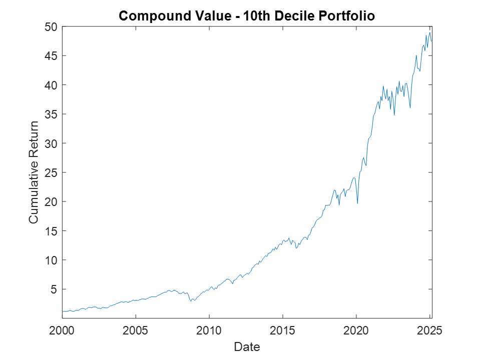
Using the model’s predicted rank scores, we form decile portfolios rebalanced monthly over a 25-year period (2000-2025), with an average turnover of 66% per month.
The top decile (Decile 10) portfolio demonstrates a Sharpe Ratio of approximately 0.8 with an annualized return of 17.8%—impressive performance that validates our approach. As shown in the cumulative return chart, performance remained consistent across different market regimes, including the 2008 financial crisis, the 2020 pandemic crash, and subsequent recovery periods.
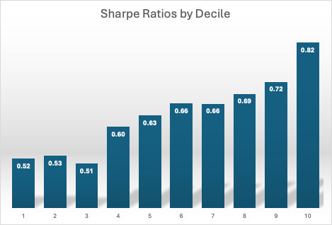
Risk-adjusted performance increases across the decile portfolios, indicating that the selected factors appear to provide real explanatory power:
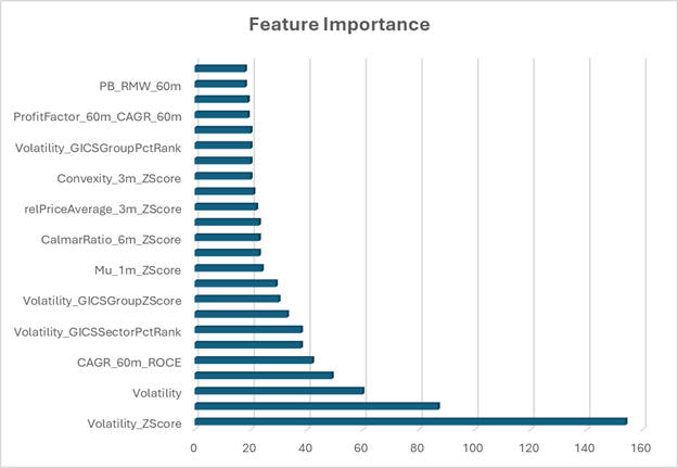
Looking at the feature importance chart, the most significant features include:
- Technical features:
- Volatility metrics dominate with “Volatility_ZScore” being the most important feature by a wide margin
- “Mu_1m_ZScore” (1-month return z-score)
- “relPriceAverage_3m_ZScore” (3-month relative price average)
- “Convexity_3m_ZScore” (price path convexity over 3 months)
- Fundamental features:
- “PB_RMW_60m” (Price-to-Book adjusted for profitability over 60 months)
- Interaction terms
- “CAGR_60m_ROCE” (compound annual growth rate combined with return on capital employed)
- ProfitFactor_60m_CAGR_60m” (interaction between profit factor and growth)
- Cross-sectional features:
- “CalmarRatio_6m_ZScore” (risk-adjusted return metric)
- “Volatility_GICSSectorPctRank” (sector-normalized volatility percentile rank)
Our model was trained on data from 1995-1999 and validated on an independent holdout set before final out-of-sample testing from 2000-2025, in which the model is updated every 60 months.
This rigorous approach to validation ensures that our performance metrics reflect realistic expectations rather than in-sample overfitting.
This diverse feature set confirms that durable alpha generation requires the integration of multiple orthogonal signals unified under a common ranking framework—precisely what our Python Equities Entity Store facilitates. The dominance of volatility-related features suggests that risk management is a critical component of the model’s predictive power.
Package Structure and Implementation
The Python EES is organized as follows:
equityentity/
├── __init__.py
├── features/
│ ├── loader.py # Load features from HDF5
│ ├── preprocess.py # Standardization, neutralization, filtering
│ └── labels.py # Target generation (e.g., IR@1m)
├── models/
│ └── ranker.py # LambdaMART, LightGBM ranking models
├── portfolio/
│ └── constructor.py # Create portfolios from rank scores
├── backtest/
│ └── evaluator.py # Sharpe, IR, turnover, hit rate
└── entity/ # Optional metadata (JSON to dataclass)
├── equity.py
├── etf.py
└── index.py
Code Example: Ranking Model Training
Here’s how the ranking model module works, leveraging LightGBM’s LambdaMART implementation:
class RankModel:

    def __init__(self, max_depth=4, num_leaves=32, learning_rate=0.1, n_estimators=500,
use_gpu=True, feature_names=None):

        self.params = {
            "objective": "lambdarank",
            "max_depth": max_depth,
            "num_leaves": num_leaves,
            "learning_rate": learning_rate,
            "n_estimators": n_estimators,
            "device": "gpu" if use_gpu else "cpu",
            "verbose": -1,
            "max_position": 50
        }

        self.model = None
        self.feature_names = feature_names if feature_names is not None else []

    def train(self, features, labels):

        # Reshape features and labels for LambdaMART format
        n_months, n_stocks, n_features = features.shape
        X = features.reshape(-1, n_features)
        y = labels.reshape(-1)
        group = [n_stocks] * n_months
        train_data = lgb.Dataset(X, label=y, group=group, feature_name=self.feature_names)
        self.model = lgb.train(self.params, train_data)
Portfolio Construction
The system seamlessly transitions from predictive scores to portfolio allocation with built-in transaction cost modeling:
# Portfolio construction with transaction cost awareness
def construct_portfolios(self):

    n_months, n_stocks = self.pred_scores.shape

    for t in range(n_months):

        # Get predictions and forward returns
        scores = self.pred_scores[t]
        returns_t = self.returns[min(t + 1, n_months - 1)]

        # Select top and bottom deciles
        sorted_idx = np.argsort(scores)
        long_idx = sorted_idx[-n_decile:]
        short_idx = sorted_idx[:n_decile]

        # Calculate transaction costs from portfolio turnover
        curr_long_symbols = set(symbols_t[long_idx])
        curr_short_symbols = set(symbols_t[short_idx])
        long_trades = len(curr_long_symbols.symmetric_difference(self.prev_long_symbols))
        short_trades = len(curr_short_symbols.symmetric_difference(self.prev_short_symbols))

        tx_cost_long = self.tx_cost * long_trades
        tx_cost_short = self.tx_cost * short_trades

        # Calculate net returns with costs
        long_ret = long_raw - tx_cost_long
        short_ret = -short_raw - tx_cost_short - self.loan_cost
Complete Workflow Example
The package is designed for intuitive workflows with minimal boilerplate. Here’s how simple it is to get started:
from equityentity.features import FeatureLoader, LabelGenerator
from equityentity.models import LambdaMARTRanker
from equityentity.portfolio import DecilePortfolioConstructor

# Load features with point-in-time awareness
loader = FeatureLoader(hdf5_path='equity_features.h5')
features = loader.load_features(start_date='2010-01-01', end_date='2025-01-01')

# Generate IR_1m labels
label_gen = LabelGenerator(benchmark='sector_returns')
labels = label_gen.create_information_ratio(forward_period='1M')

# Train a ranking model
ranker = LambdaMARTRanker(n_estimators=500, learning_rate=0.05)
ranker.fit(features, labels)

# Create portfolios from predictions
constructor = DecilePortfolioConstructor(rebalance_freq='M')
portfolios = constructor.create_from_scores(ranker.predict(features))

# Evaluate performance
performance = portfolios['decile_10'].evaluate()
print(f"Sharpe Ratio: {performance['sharpe_ratio']:.2f}")
print(f"Information Ratio: {performance['information_ratio']:.2f}")
print(f"Annualized Return: {performance['annualized_return']*100:.1f}%")
The package supports both configuration file-based workflows for production use and interactive Jupyter notebook exploration. Output formats include pandas DataFrames, JSON for web applications, and HDF5 for efficient storage of results.
Why Start with Cross-Sectional ML?
While Mathematica’s EntityStore emphasized symbolic navigation and knowledge representation, Python excels at algorithmic learning and numerical computation at scale. Beginning with the HDF5 dataset enables immediate application by quantitative researchers, ML specialists, and strategy developers interested in:
- Exploring sophisticated feature engineering across time horizons and market sectors
- Building powerful predictive ranking models with state-of-the-art ML techniques
- Constructing long-short portfolios with dynamic scoring mechanisms
- Developing robust factor models and alpha signals
And because we’ve already created metadata-rich JSON files for each entity, we can progressively integrate the symbolic structure—creating a hybrid system where machine learning capabilities complement knowledge representation.
Increasingly, quantitative researchers are integrating tools like LangChain, GPT-based agents, and autonomous research pipelines to automate idea generation, feature testing, and code execution. The structured design of the Python Equities Entity Store—with its modularity, metadata integration, and time-consistent features—makes it ideally suited for use as a foundation in LLM-driven quantitative workflows.
Competitive Pricing and Value
While alternative platforms in this space typically come with significant cost barriers, we’ve positioned the Python Equities Entity Store to be accessible to firms of all sizes:
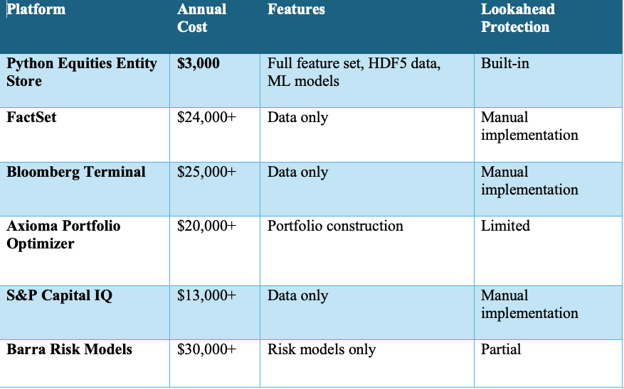
While open-source platforms like QuantConnect, Zipline, and Backtrader provide accessible backtesting environments, they often lack the scale, granularity, and point-in-time feature control required for advanced cross-sectional ML strategies. The Python Equities Entity Store fills this gap—offering industrial-strength data infrastructure, lookahead protection, and extensibility without the steep cost of commercial platforms.
Unlike these competitors that often require multiple subscriptions to achieve similar functionality, Python Equities Entity Store provides an integrated solution at a fraction of the cost. This pricing strategy reflects our commitment to democratizing access to institutional-grade quantitative tools.
Next Steps
We’re excited to announce our roadmap for the Python Equities Entity Store:
- July 2025 Release: The official launch of our HDF5-compatible package, complete with:
- Comprehensive documentation and API reference
- Jupyter notebooks demonstrating key workflows from data loading to portfolio construction
- Example strategies showcasing the system’s capabilities across different market regimes
- Performance benchmarks and baseline models with full backtest history
- Python package available via PyPI (pip install equityentity)
- Docker container with pre-loaded example datasets
- Q3 2025: Integration of the symbolic entity framework, allowing seamless navigation between quantitative features and qualitative metadata
- Q4 2025: Extension to additional asset classes and alternative data sources, expanding the system’s analytical scope
- Early 2026: Launch of a cloud-based computational environment for collaboration and strategy sharing
Accessing the Python Equities Entity Store
As a special promotion, existing users of the current Mathematica Equities Entity Store Enterprise Edition will be given free access to the Python version on launch.
So, if you sign up now for the Enterprise Edition you will receive access to both the existing Mathematica version and the new Python version as soon as it is released.
After the launch of the Python Equities Entity Store, each product will be charged individually. So this limited time offer represents a 50% discount.
See our web site for pricing details: https://store.equityanalytics.store/equities-entity-store
Conclusion
By prioritizing scalable feature datasets and sophisticated ranking models, the Python version of the Equities Entity Store positions itself as an indispensable tool for modern equity research. It bridges the gap between raw data and actionable insights, combining the power of machine learning with the structure of knowledge representation.
The Python Equities Entity Store represents a significant step forward in quantitative finance tooling—enabling faster iteration, more robust models, and ultimately, better investment decisions.