Futures Archives - Page 2 of 4 - QUANTITATIVE RESEARCH AND TRADING

February 18, 2020

Futures WealthBuilder – June 2017: +4.4%

The Futures WealthBuilder product is an algorithmic CTA strategy that trades several highly liquid futures contracts using machine learning algorithms. More details about the strategy are given in this blog post.

We offer a version of the strategy on the Collective 2 site (see here for details) that the user can subscribe to for a very modest fee of only $149 per month. The Collective 2 version of the strategy is unlikely to perform as well as the product we offer in our Systematic Strategies Fund, which trades a much wider range of futures products. But the strategy is off to an excellent start, making +4.4% in June and is now up 6.7% since inception in May. In June the strategy made profitable trades in US Bonds, Euro F/X and VIX futures, and the last seven trades in a row have been winners.

You can find full details of the strategy, including a listing of all of the trades, on the Collective 2 site.

Subscribers can sign up for a free, seven day trial and thereafter they can choose to trade the strategy automatically in their own brokerage account, using the Collective 2 api.

January 14, 2020

Futures WealthBuilder

We are launching a new product, the Futures WealthBuilder, a CTA system that trades futures contracts in several highly liquid financial and commodity markets, including SP500 EMinis, Euros, VIX, Gold, US Bonds, 10-year and five-year notes, Corn, Natural Gas and Crude Oil. Each component strategy uses a variety of machine learning algorithms to detect trends, seasonal effects and mean-reversion. We develop several different types of model for each market, and deploy them according to their suitability for current market conditions.

Performance of the strategy (net of fees) since 2013 is detailed in the charts and tables below. Notable features include a Sharpe Ratio of just over 2, an annual rate of return of 190% on an account size of $50,000, and a maximum drawdown of around 8% over the last three years. It is worth mentioning, too, that the strategy produces approximately equal rates of return on both long and short trades, with an overall profit factor above 2.

Low Correlation

Despite a high level of correlation between several of the underlying markets, the correlation between the component strategies of Futures WealthBuilder are, in the majority of cases, negligibly small (with a few exceptions, such as the high correlation between the 10-year and 5-year note strategies). This accounts for the relative high level of return in relation to portfolio risk, as measured by the Sharpe Ratio. We offer strategies in both products chiefly as a mean of providing additional liquidity, rather than for their diversification benefit.

Strategy Robustness

Strategy robustness is a key consideration in the design stage. We use Monte Carlo simulation to evaluate scenarios not seen in historical price data in order to ensure consistent performance across the widest possible range of market conditions. Our methodology introduces random fluctuations to historical prices, increasing or decreasing them by as much as 30%. We allow similar random fluctuations in that value strategy parameters, to ensure that our models perform consistently without being overly-sensitive to the specific parameter values we have specified. Finally, we allow the start date of each sub-system to vary randomly by up to a year.

The effect of these variations is to produce a wide range of outcomes in terms of strategy performance. We focus on the 5% worst outcomes, ranked by profitability, and select only those strategies whose performance is acceptable under these adverse scenarios. In this way we reduce the risk of overfitting the models while providing more realistic expectations of model performance going forward. This procedure also has the effect of reducing portfolio tail risk, and the maximum peak-to-valley drawdown likely to be produced by the strategy in future.

Futures WealthBuilder on Collective 2

We will be running a variant of the Futures WealthBuilder strategy on the Collective 2 site, using a subset of the strategy models in several futures markets(see this page for details). Subscribers will be able to link and auto-trade the strategy in their own account, assuming they make use of one of the approved brokerages which include Interactive Brokers, MB Trading and several others.

Obviously the performance is unlikely to be as good as the complete strategy, since several component sub-strategies will not be traded on Collective 2. However, this does give the subscriber the option to trial the strategy in simulation before plunging in with real money.

November 12, 2019

HFT VIX Scalper Leads on Collective2

Our high frequency VIX scalping strategy is now the #1 top performing strategy on Collective2, with returns of over 2700% since April 2016 with a Sharpe Ratio above 10 and Profit Factor of 2.8.

For more background on HFT scalping strategies see the following post:

http://jonathankinlay.com/2014/05/the-mathematics-of-scalping/

October 8, 2019October 8, 2019

High Frequency Scalping Strategies

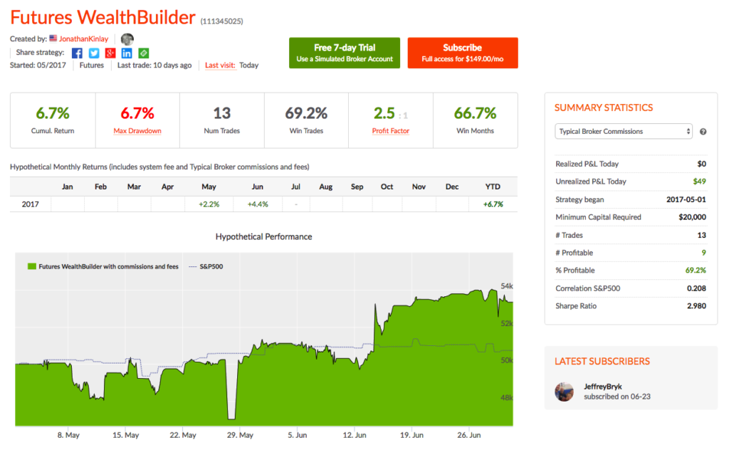
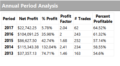
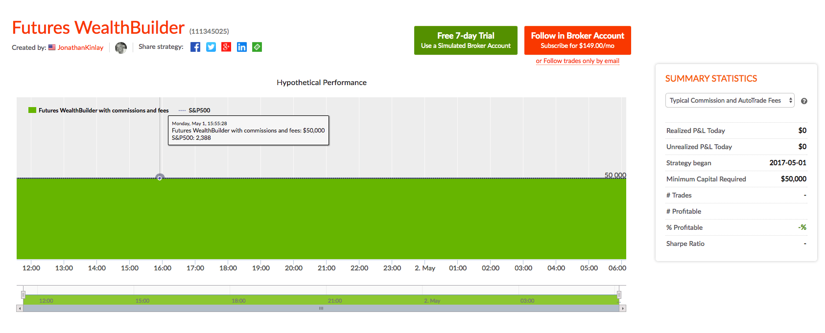
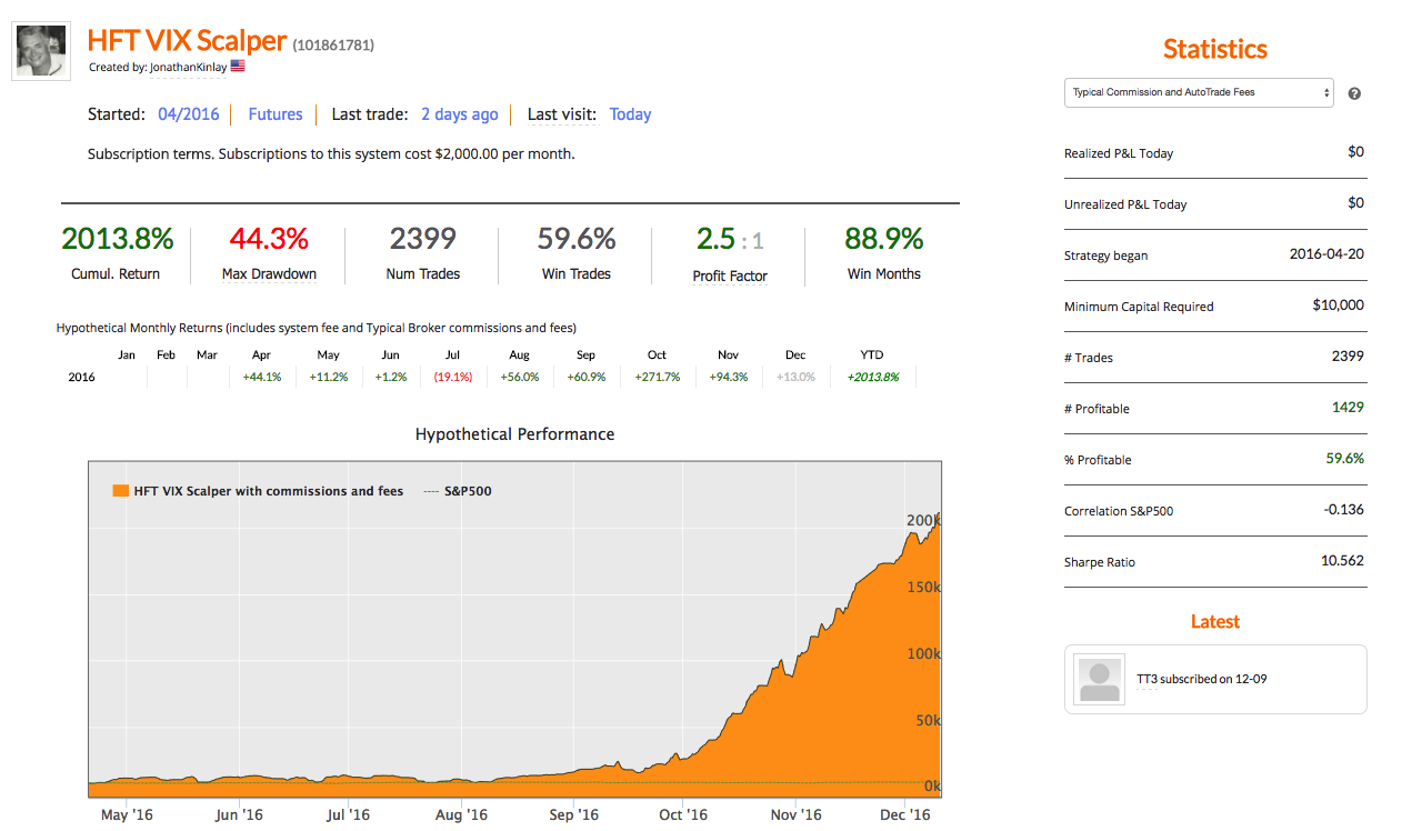
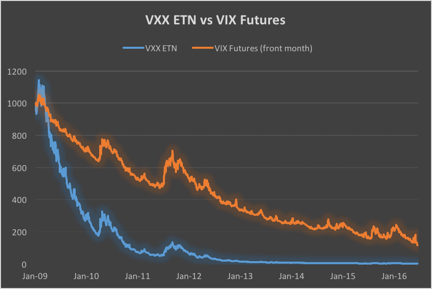
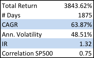
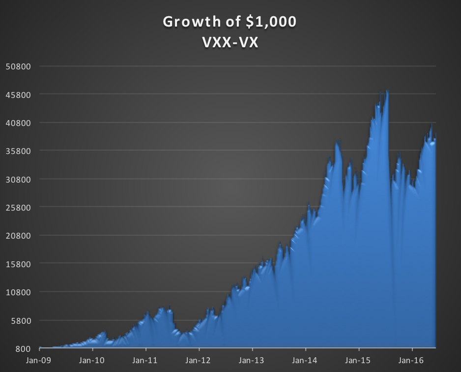
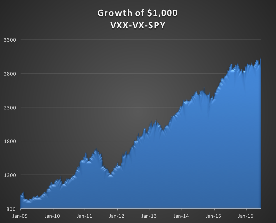
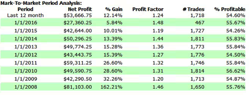
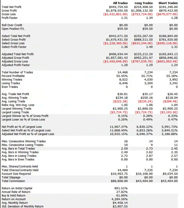
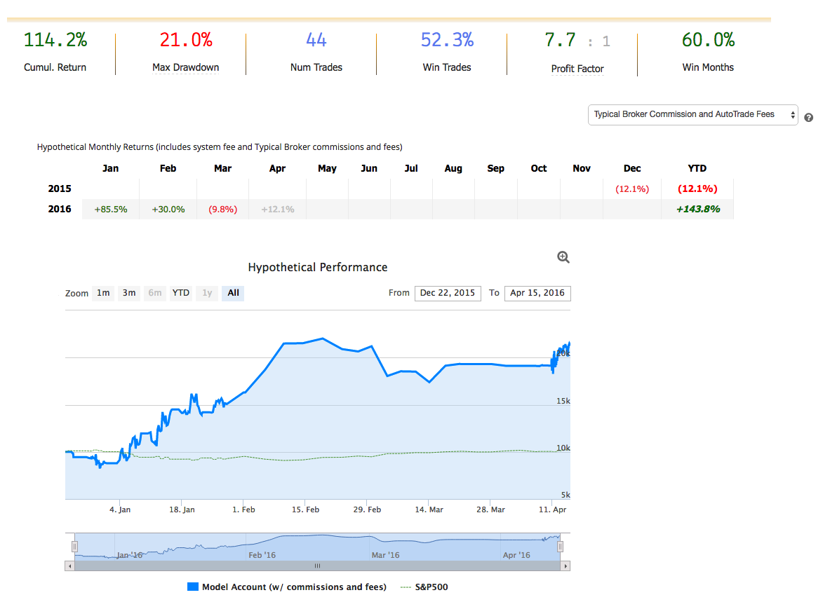
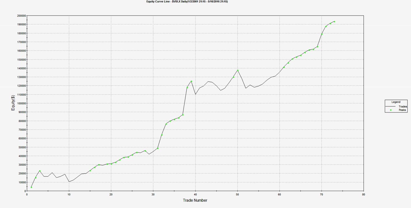
HFT scalping strategies enjoy several highly desirable characteristics, compared to low frequency strategies. A case in point is our scalping strategy in VIX futures, currently running on the Collective2 web site:

The strategy is highly profitable, with a Sharpe Ratio in excess of 9 (net of transaction costs of $14 prt)
Performance is consistent and reliable, being based on a large number of trades (10-20 per day)
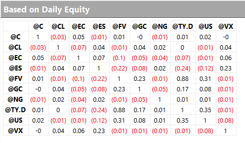
The strategy has low, or negative correlation to the underlying equity and volatility indices
There is no overnight risk

Background on HFT Scalping Strategies

The attractiveness of such strategies is undeniable. So how does one go about developing them?

It is important for the reader to familiarize himself with some of the background to high frequency trading in general and scalping strategies in particular. Specifically, I would recommend reading the following blog posts:

http://jonathankinlay.com/2015/05/high-frequency-trading-strategies/

http://jonathankinlay.com/2014/05/the-mathematics-of-scalping/

Execution vs Alpha Generation in HFT Strategies

The key to understanding HFT strategies is that execution is everything. With low frequency strategies a great deal of work goes into researching sources of alpha, often using highly sophisticated mathematical and statistical techniques to identify and separate the alpha signal from the background noise. Strategy alpha accounts for perhaps as much as 80% of the total return in a low frequency strategy, with execution making up the remaining 20%. It is not that execution is unimportant, but there are only so many basis points one can earn (or save) in a strategy with monthly turnover. By contrast, a high frequency strategy is highly dependent on trade execution, which may account for 80% or more of the total return. The algorithms that generate the strategy alpha are often very simple and may provide only the smallest of edges. However, that very small edge, scaled up over thousands of trades, is sufficient to produce a significant return. And since the risk is spread over a large number of very small time increments, the rate of return can become eye-wateringly high on a risk-adjusted basis: Sharpe Ratios of 10, or more, are commonly achieved with HFT strategies.

In many cases an HFT algorithm seeks to estimate the conditional probability of an uptick or downtick in the underlying, leaning on the bid or offer price accordingly. Provided orders can be positioned towards the front of the queue to ensure an adequate fill rate, the laws of probability will do the rest. So, in the HFT context, much effort is expended on mitigating latency and on developing techniques for establishing and maintaining priority in the limit order book. Another major concern is to monitor order book dynamics for signs that book pressure may be moving against any open orders, so that they can be cancelled in good time, avoiding adverse selection by informed traders, or a buildup of unwanted inventory.

In a high frequency scalping strategy one is typically looking to capture an average of between 1/2 to 1 tick per trade. For example, the VIX scalping strategy illustrated here averages around $23 per contract per trade, i.e. just under 1/2 a tick in the futures contract. Trade entry and exit is effected using limit orders, since there is no room to accommodate slippage in a trading system that generates less than a single tick per trade, on average. As with most HFT strategies the alpha algorithms are only moderately sophisticated, and the strategy is highly dependent on achieving an acceptable fill rate (the proportion of limit orders that are executed). The importance of achieving a high enough fill rate is clearly illustrated in the first of the two posts referenced above. So what is an acceptable fill rate for a HFT strategy?

Fill Rates

I’m going to address the issue of fill rates by focusing on a critical subset of the problem: fills that occur at the extreme of the bar, also known as “extreme hits”. These are limit orders whose prices coincide with the highest (in the case of a sell order) or lowest (in the case of a buy order) trade price in any bar of the price series. Limit orders at prices within the interior of the bar are necessarily filled and are therefore uncontroversial. But limit orders at the extremities of the bar may or may not be filled and it is therefore these orders that are the focus of attention.

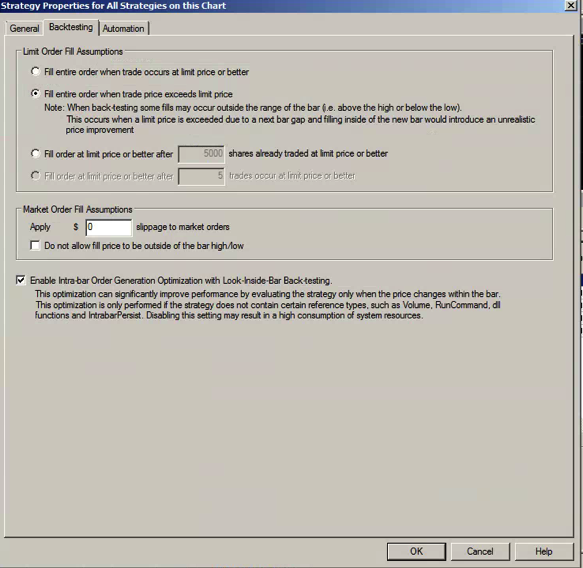
By default, most retail platform backtest simulators assume that all limit orders, including extreme hits, are filled if the underlying trades there. In other words, these systems typically assume a 100% fill rate on extreme hits. This is highly unrealistic: in many cases the high or low of a bar forms a turning point that the price series visits only fleetingly before reversing its recent trend, and does not revisit for a considerable time. The first few orders at the front of the queue will be filled, but many, perhaps the majority of, orders further down the priority order will be disappointed. If the trader is using a retail trading system rather than a HFT platform to execute his trades, his limit orders are almost always guaranteed to rest towards the back of the queue, due to the relatively high latency of his system. As a result, a great many of his limit orders – in particular, the extreme hits – will not be filled.

The consequences of missing a large number of trades due to unfilled limit orders are likely to be catastrophic for any HFT strategy. A simple test that is readily available in most backtest systems is to change the underlying assumption with regard to the fill rate on extreme hits – instead of assuming that 100% of such orders are filled, the system is able to test the outcome if limit orders are filled only if the price series subsequently exceeds the limit price. The outcome produced under this alternative scenario is typically extremely adverse, as illustrated in first blog post referenced previously.

In reality, of course, neither assumption is reasonable: it is unlikely that either 100% or 0% of a strategy’s extreme hits will be filled – the actual fill rate will likely lie somewhere between these two outcomes. And this is the critical issue: at some level of fill rate the strategy will move from profitability into unprofitability. The key to implementing a HFT scalping strategy successfully is to ensure that the execution falls on the right side of that dividing line.

Implementing HFT Scalping Strategies in Practice

One solution to the fill rate problem is to spend millions of dollars building HFT infrastructure. But for the purposes of this post let’s assume that the trader is confined to using a retail trading platform like Tradestation or Interactive Brokers. Are HFT scalping systems still feasible in such an environment? The answer, surprisingly, is a qualified yes – by using a technique that took me many years to discover.

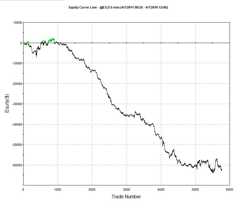
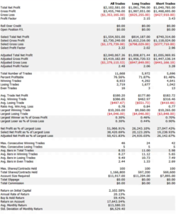
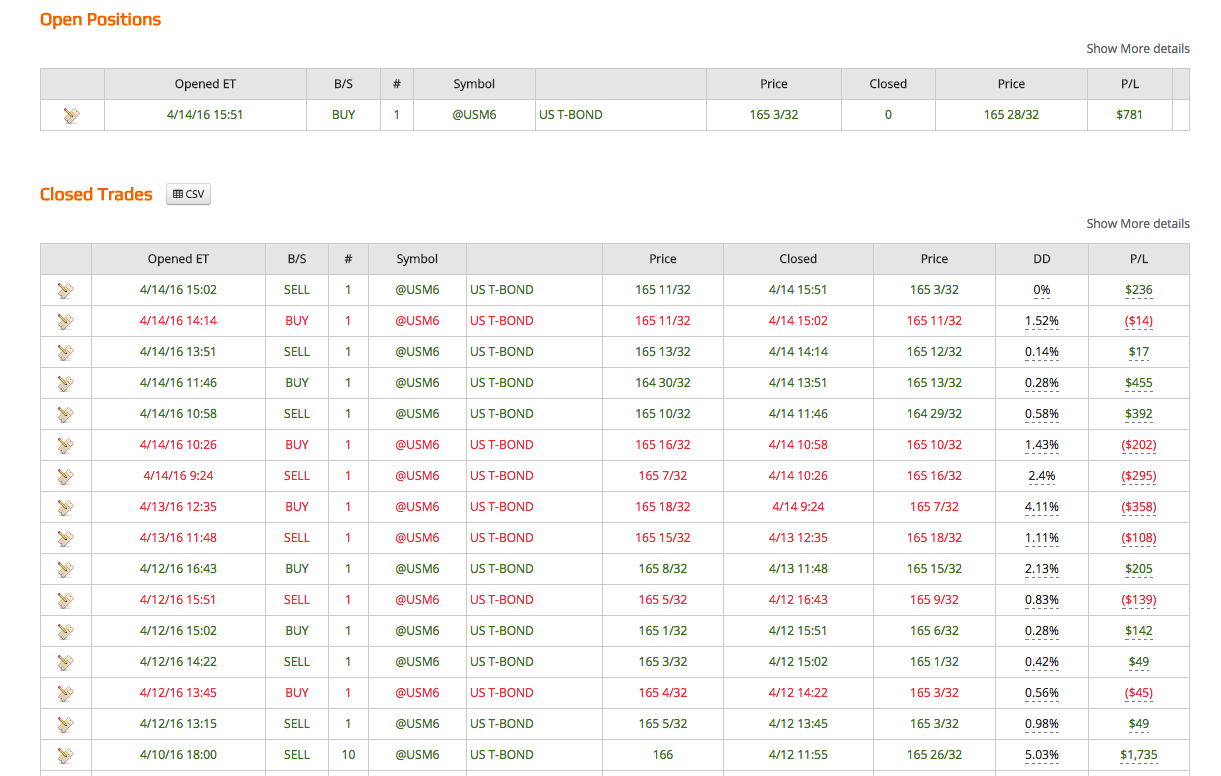
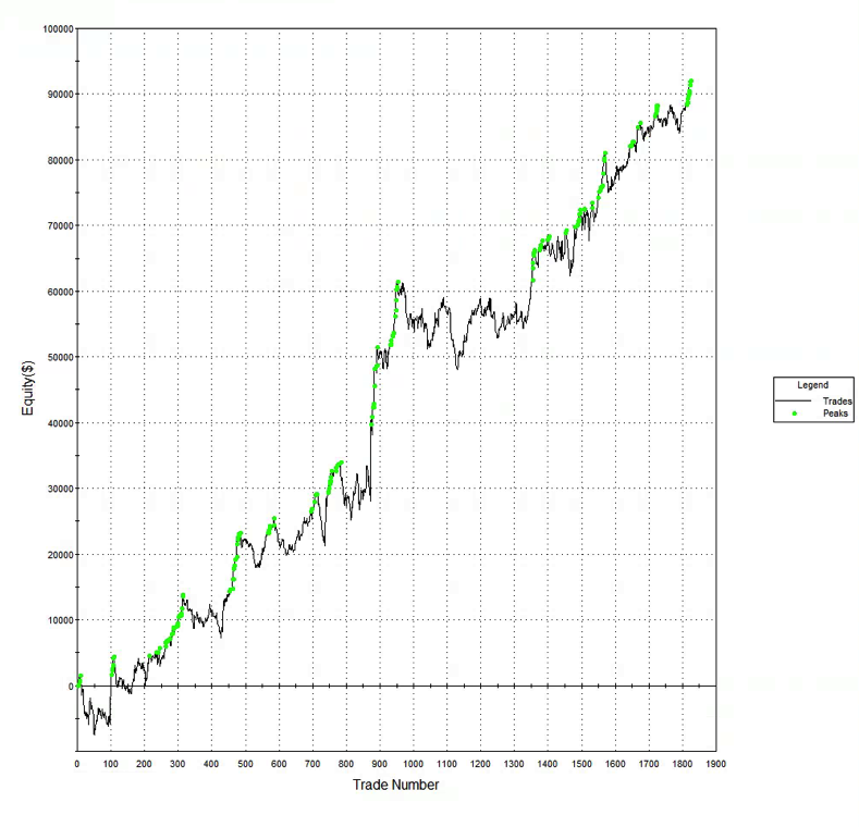
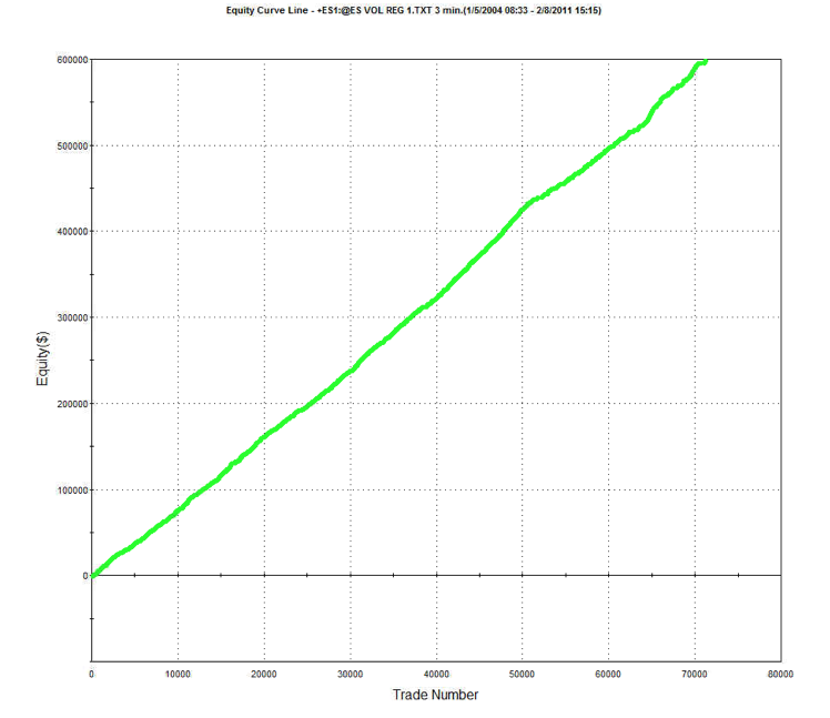
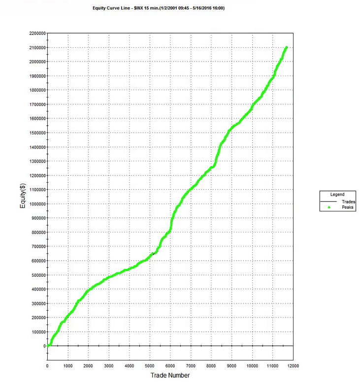
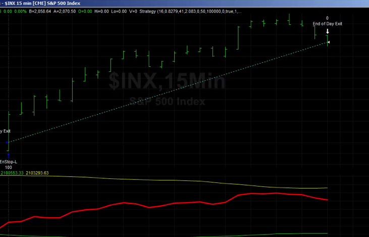
To illustrate the method I will use the following HFT scalping system in the E-Mini S&P500 futures contract. The system trades the E-Mini futures on 3 minute bars, with an average hold time of 15 minutes. The average trade is very low – around $6, net of commissions of $8 prt. But the strategy appears to be highly profitable ,due to the large number of trades – around 50 to 60 per day, on average.

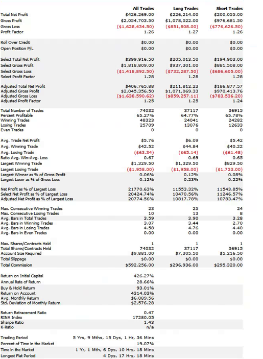
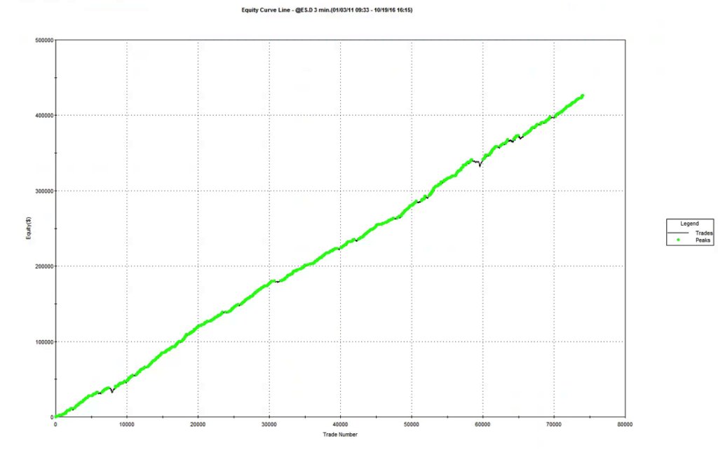
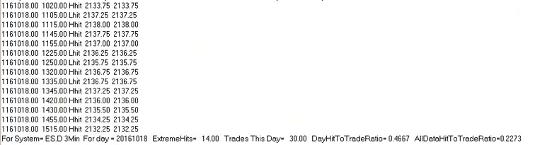
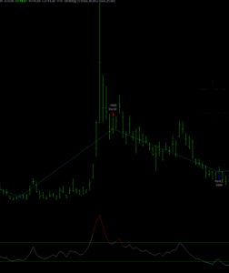
So far so good. But the critical issue is the very large number of extreme hits produced by the strategy. Take the trading activity on 10/18 as an example (see below). Of 53 trades that day, 25 (47%) were extreme hits, occurring at the high or low price of the 3-minute bar in which the trade took place.

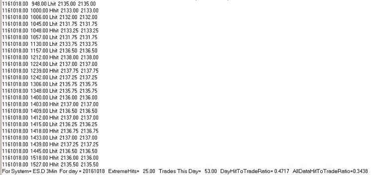
Overall, the strategy extreme hit rate runs at 34%, which is extremely high. In reality, perhaps only 1/4 or 1/3 of these orders will actually execute – meaning that remainder, amounting to around 20% of the total number of orders, will fail. A HFT scalping strategy cannot hope to survive such an outcome. Strategy profitability will be decimated by a combination of missed, profitable trades and losses on trades that escalate after an exit order fails to execute.

So what can be done in such a situation?

Manual Override, MIT and Other Interventions

One approach that will not work is to assume naively that some kind of manual oversight will be sufficient to correct the problem. Let’s say the trader runs two versions of the system side by side, one in simulation and the other in production. When a limit order executes on the simulation system, but fails to execute in production, the trader might step in, manually override the system and execute the trade by crossing the spread. In so doing the trader might prevent losses that would have occurred had the trade not been executed, or force the entry into a trade that later turns out to be profitable. Equally, however, the trader might force the exit of a trade that later turns around and moves from loss into profit, or enter a trade that turns out to be a loser. There is no way for the trader to know, ex-ante, which of those scenarios might play out. And the trader will have to face the same decision perhaps as many as twenty times a day. If the trader is really that good at picking winners and cutting losers he should scrap his trading system and trade manually!

An alternative approach would be to have the trading system handle the problem, For example, one could program the system to convert limit orders to market orders if a trade occurs at the limit price (MIT), or after x seconds after the limit price is touched. Again, however, there is no way to know in advance whether such action will produce a positive outcome, or an even worse outcome compared to leaving the limit order in place.

In reality, intervention, whether manual or automated, is unlikely to improve the trading performance of the system. What is certain, however, is that by forcing the entry and exit of trades that occur around the extreme of a price bar, the trader will incur additional costs by crossing the spread. Incurring that cost for perhaps as many as 1/3 of all trades, in a system that is producing, on average less than half a tick per trade, is certain to destroy its profitability.

Successfully Implementing HFT Strategies on a Retail Platform

For many years I assumed that the only solution to the fill rate problem was to implement scalping strategies on HFT infrastructure. One day, I found myself asking the question: what would happen if we slowed the strategy down? Specifically, suppose we took the 3-minute E-Mini strategy and ran it on 5-minute bars?

My first realization was that the relative simplicity of alpha-generation algorithms in HFT strategies is an advantage here. In a low frequency context, the complexity of the alpha extraction process mitigates its ability to generalize to other assets or time-frames. But HFT algorithms are, by and large, simple and generic: what works on 3-minute bars for the E-Mini futures might work on 5-minute bars in E-Minis, or even in SPY. For instance, if the essence of the algorithm is something as simple as: “buy when the price falls by more than x% below its y-bar moving average”, that approach might work on 3-minute, 5-minute, 60-minute, or even daily bars.

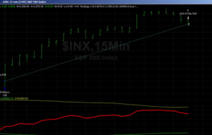
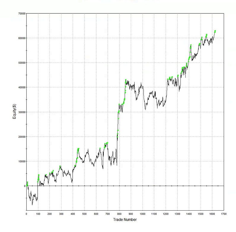
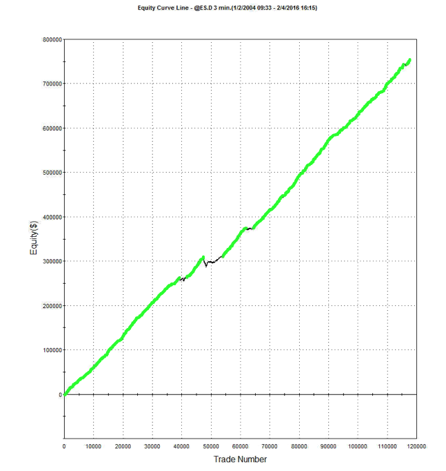
So what happens if we run the E-mini scalping system on 5-minute bars instead of 3-minute bars?

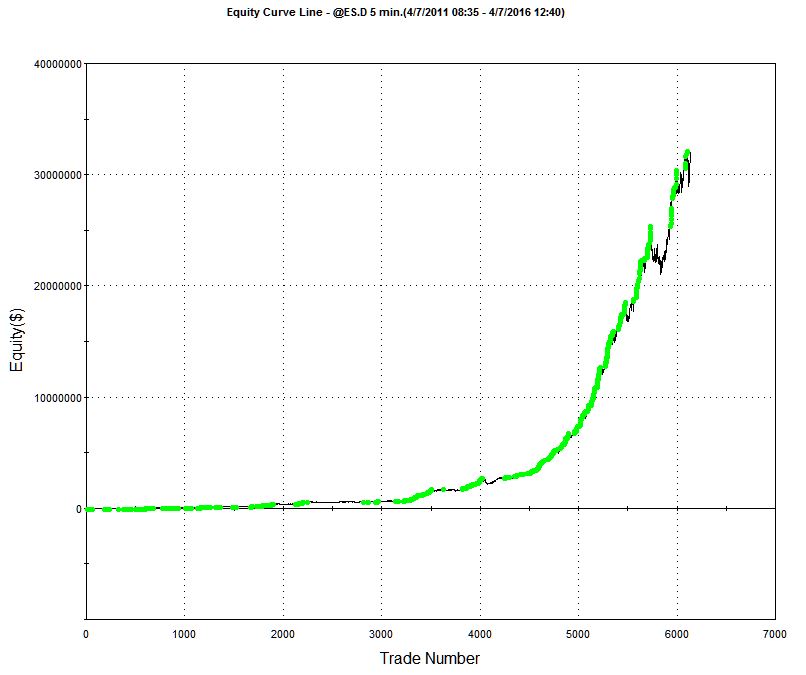
Obviously the overall profitability of the strategy is reduced, in line with the lower number of trades on this slower time-scale. But note that average trade has increased and the strategy remains very profitable overall.

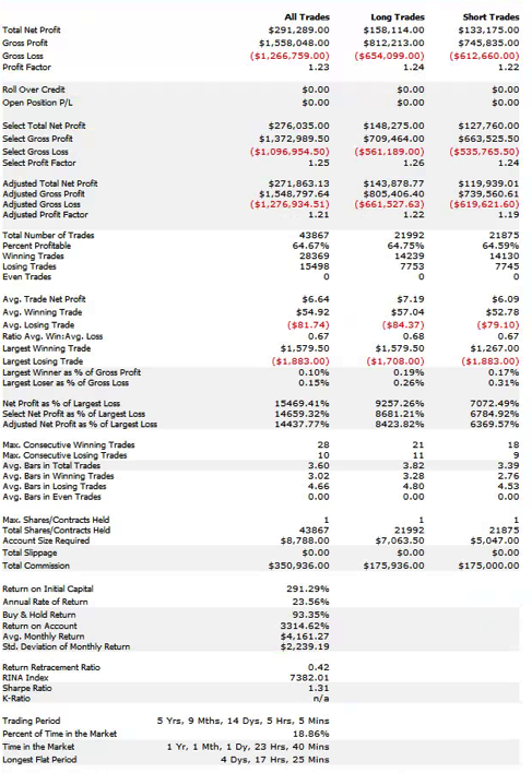
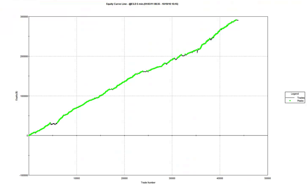
More importantly, the average extreme hit rate has fallen from 34% to 22%.

Hence, not only do we get fewer, slightly more profitable trades, but a much lower proportion of them occur at the extreme of the 5-minute bars. Consequently the fill-rate issue is less critical on this time frame.

Of course, one can continue this process. What about 10-minute bars, or 30-minute bars? What one tends to find from such experiments is that there is a time frame that optimizes the trade-off between strategy profitability and fill rate dependency.

However, there is another important factor we need to elucidate. If you examine the trading record from the system you will see substantial variation in the extreme hit rate from day to day (for example, it is as high as 46% on 10/18, compared to the overall average of 22%). In fact, there are significant variations in the extreme hit rate during the course of each trading day, with rates rising during slower market intervals such as from 12 to 2pm. The important realization that eventually occurred to me is that, of course, what matters is not clock time (or “wall time” in HFT parlance) but trade time: i.e. the rate at which trades occur.

Wall Time vs Trade Time

What we need to do is reconfigure our chart to show bars comprising a specified number of trades, rather than a specific number of minutes. In this scheme, we do not care whether the elapsed time in a given bar is 3-minutes, 5-minutes or any other time interval: all we require is that the bar comprises the same amount of trading activity as any other bar. During high volume periods, such as around market open or close, trade time bars will be shorter, comprising perhaps just a few seconds. During slower periods in the middle of the day, it will take much longer for the same number of trades to execute. But each bar represents the same level of trading activity, regardless of how long a period it may encompass.

How do you decide how may trades per bar you want in the chart?

As a rule of thumb, a strategy will tolerate an extreme hit rate of between 15% and 25%, depending on the daily trade rate. Suppose that in its original implementation the strategy has an unacceptably high hit rate of 50%. And let’s say for illustrative purposes that each time-bar produces an average of 1, 000 contracts. Since volatility scales approximately with the square root of time, if we want to reduce the extreme hit rate by a factor of 2, i.e. from 50% to 25%, we need to increase the average number of trades per bar by a factor of 2^2, i.e. 4. So in this illustration we would need volume bars comprising 4,000 contracts per bar. Of course, this is just a rule of thumb – in practice one would want to implement the strategy of a variety of volume bar sizes in a range from perhaps 3,000 to 6,000 contracts per bar, and evaluate the trade-off between performance and fill rate in each case.

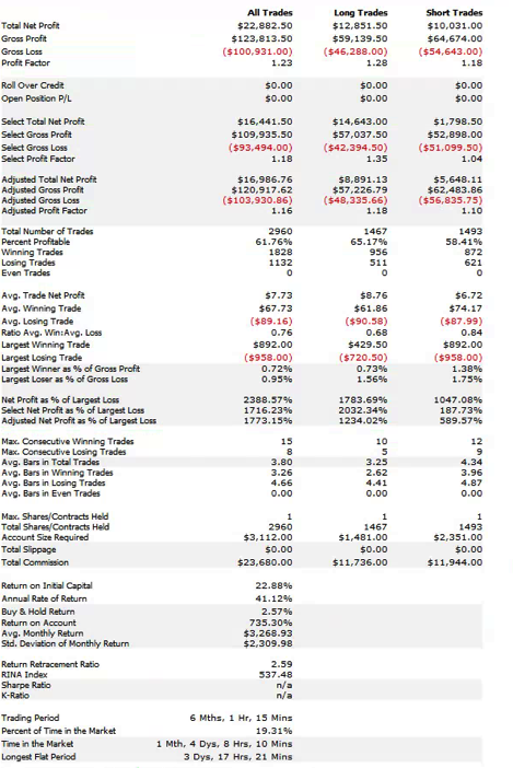
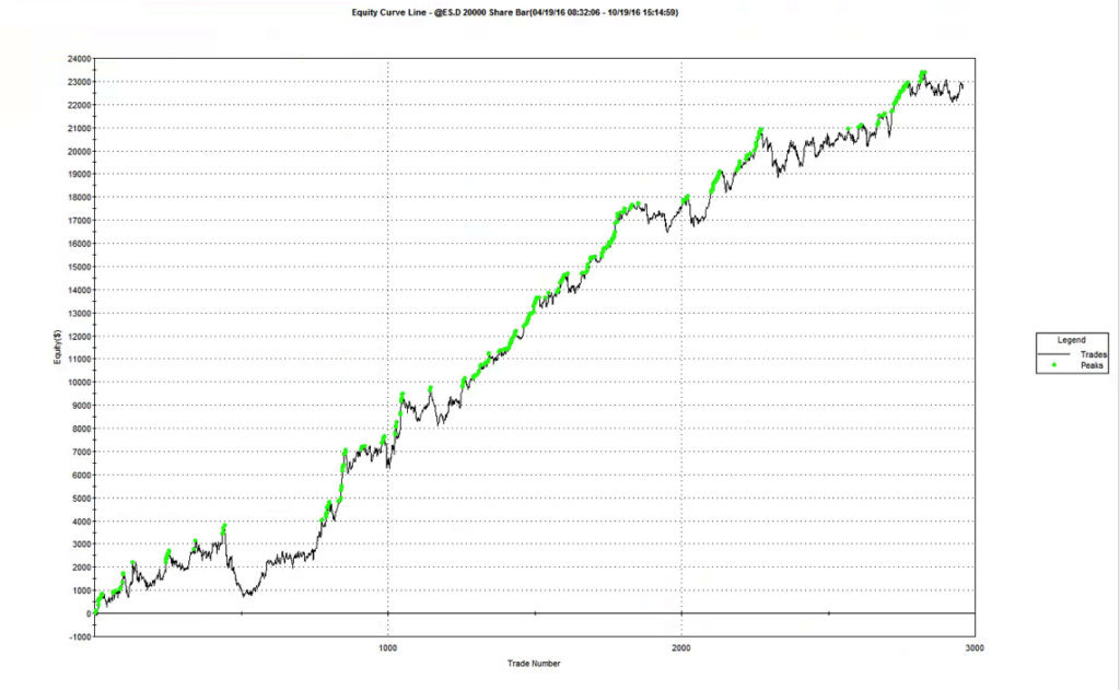
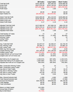
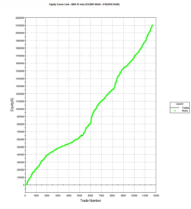
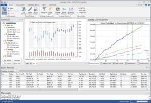
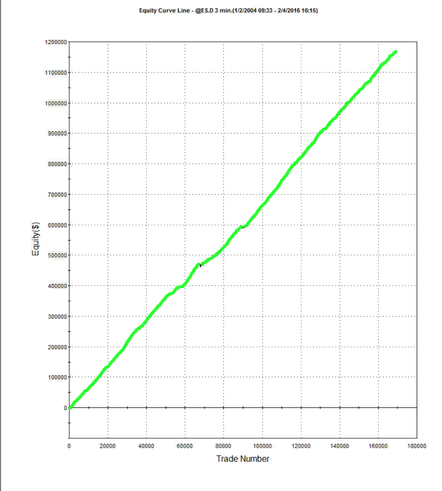
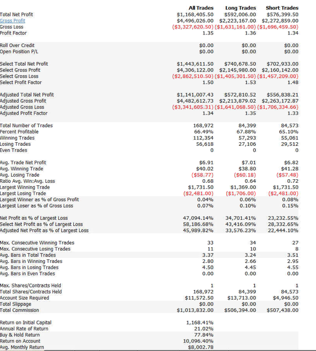
Using this approach, we arrive at a volume bar configuration for the E-Mini scalping strategy of 20,000 contracts per bar. On this “time”-frame, trading activity is reduced to around 20-25 trades per day, but with higher win rate and average trade size. More importantly, the extreme hit rate runs at a much lower average of 22%, which means that the trader has to worry about maybe only 4 or 5 trades per day that occur at the extreme of the volume bar. In this scenario manual intervention is likely to have a much less deleterious effect on trading performance and the strategy is probably viable, even on a retail trading platform.

(Note: the results below summarize the strategy performance only over the last six months, the time period for which volume bars are available).

Concluding Remarks

We have seen that is it feasible in principle to implement a HFT scalping strategy on a retail platform by slowing it down, i.e. by implementing the strategy on bars of lower frequency. The simplicity of many HFT alpha generation algorithms often makes them robust to generalization across time frames (and sometimes even across assets). An even better approach is to use volume bars, or trade-time, to implement the strategy. You can estimate the appropriate bar size using the square root of time rule to adjust the bar volume to produce the requisite fill rate. An extreme hit rate if up to 25% may be acceptable, depending on the daily trade rate, although a hit rate in the range of 10% to 15% would typically be ideal.

Finally, a word about data. While necessary compromises can be made with regard to the trading platform and connectivity, the same is not true for market data, which must be of the highest quality, both in terms of timeliness and completeness. The reason is self evident, especially if one is attempting to implement a strategy in trade time, where the integrity and latency of market data is crucial. In this context, using the data feed from, say, Interactive Brokers, for example, simply will not do – data delivered in 500ms packets in entirely unsuited to the task. The trader must seek to use the highest available market data feed that he can reasonably afford.

That caveat aside, one can conclude that it is certainly feasible to implement high volume scalping strategies, even on a retail trading platform, providing sufficient care is taken with the modeling and implementation of the system.

September 17, 2019

High Frequency Futures Scalping Strategies Update

July 16, 2019

Developing A Volatility Carry Strategy

By way of introduction we begin by reviewing a well known characteristic of the iPath S&P 500 VIX ST Futures ETN (NYSEArca:VXX). In common with other long-volatility ETF /ETNs, VXX has a tendency to decline in value due to the upward sloping shape of the forward volatility curve. The chart below which illustrates the fall in value of the VXX, together with the front-month VIX futures contract, over the period from 2009.

This phenomenon gives rise to opportunities for “carry” strategies, wherein a long volatility product such as VXX is sold in expectation that it will decline in value over time. Such strategies work well during periods when volatility futures are in contango, i.e. when the longer dated futures contracts have higher prices than shorter dated futures contracts and the spot VIX Index, which is typically the case around 70% of the time. An analogous strategy in the fixed income world is known as “riding down the yield curve”. When yield curves are upward sloping, a fixed income investor can buy a higher-yielding bill or bond in the expectation that the yield will decline, and the price rise, as the security approaches maturity. Quantitative easing put paid to that widely utilized technique, but analogous strategies in currency and volatility markets continue to perform well.

The challenge for any carry strategy is what happens when the curve inverts, as futures move into backwardation, often giving rise to precipitous losses. A variety of hedging schemes have been devised that are designed to mitigate the risk. For example, one well-known carry strategy in VIX futures entails selling the front month contract and hedging with a short position in an appropriate number of E-Mini S&P 500 futures contracts. In this case the hedge is imperfect, leaving the investor the task of managing a significant basis risk.

The chart of the compounded value of the VXX and VIX futures contract suggests another approach. While both securities decline in value over time, the fall in the value of the VXX ETN is substantially greater than that of the front month futures contract. The basic idea, therefore, is a relative value trade, in which we purchase VIX futures, the better performing of the pair, while selling the underperforming VXX. Since the value of the VXX is determined by the value of the front two months VIX futures contracts, the hedge, while imperfect, is likely to entail less basis risk than is the case for the VIX-ES futures strategy.

Another way to think about the trade is this: by combining a short position in VXX with a long position in the front-month futures, we are in effect creating a residual exposure in the value of the second month VIX futures contract relative to the first. So this is a strategy in which we are looking to capture volatility carry, not at the front of the curve, but between the first and second month futures maturities. We are, in effect, riding down the belly of volatility curve.

The Relationship between VXX and VIX Futures

Let’s take a look at the relationship between the VXX and front month futures contract, which I will hereafter refer to simply as VX. A simple linear regression analysis of VXX against VX is summarized in the tables below, and confirms two features of their relationship.

Firstly there is a strong, statistically significant relationship between the two (with an R-square of 75% ) – indeed, given that the value of the VXX is in part determined by VX, how could there not be?

Secondly, the intercept of the regression is negative and statistically significant. We can therefore conclude that the underperformance of the VXX relative to the VX is not just a matter of optics, but is a statistically reliable phenomenon. So the basic idea of selling the VXX against VX is sound, at least in the statistical sense.

Constructing the Initial Portfolio

In constructing our theoretical portfolio, I am going to gloss over some important technical issues about how to construct the optimal hedge and simply assert that the best one can do is apply a beta of around 1.2, to produce the following outcome:

While broadly positive, with an information ratio of 1.32, the strategy performance is a little discouraging, on several levels. Firstly, the annual volatility, at over 48%, is uncomfortably high. Secondly, the strategy experiences very substantial drawdowns at times when the volatility curve inverts, such as in August 2015 and January 2016. Finally, the strategy is very highly correlated with the S&P500 index, which may be an important consideration for investors looking for ways to diversity their stock portfolio risk.

Exploiting Calendar Effects

We will address these issues in short order. Firstly, however, I want to draw attention to an interesting calendar effect in the strategy (using a simple pivot table analysis).

As you can see from the table above, the strategy returns in the last few days of the calendar month tend to be significantly below zero.

The cause of the phenomenon has to do with the way the VXX is constructed, but the important point here is that, in principle, we can utilize this effect to our advantage, by reversing the portfolio holdings around the end of the month. This simple technique produces a significant improvement in strategy returns, while lowering the correlation:

Reducing Portfolio Risk and Correlation

We can now address the issue of the residual high level of strategy volatility, while simultaneously reducing the strategy correlation to a much lower level. We can do this in a straightforward way by adding a third asset, the SPDR S&P 500 ETF Trust (NYSEArca:SPY), in which we will hold a short position, to exploit the negative correlation of the original portfolio.

We then adjust the portfolio weights to maximize the risk-adjusted returns, subject to limits on the maximum portfolio volatility and correlation. For example, setting a limit of 10% for both volatility and correlation, we achieve the following result (with weights -0.37 0.27 -0.65 for VXX, VX and SPY respectively):

Compared to the original portfolio, the new portfolio’s performance is much more benign during the critical period from Q2-2015 to Q1-2016 and while there remain several significant drawdown periods, notably in 2011, overall the strategy is now approaching an investable proposition, with an information ratio of 1.6 and annual volatility of 9.96% and correlation of 0.1.

Other configurations are possible, of course, and the risk-adjusted performance can be improved, depending on the investor’s risk preferences.

Portfolio Rebalancing

There is an element of curve-fitting in the research process as described so far, in as much as we are using all of the available data to July 2016 to construct a portfolio with the desired characteristics. In practice, of course, we will be required to rebalance the portfolio on a periodic basis, re-estimating the optimal portfolio weights as new data comes in. By way of illustration, the portfolio was re-estimated using in-sample data to the end of Feb, 2016, producing out-of-sample results during the period from March to July 2016, as follows:

A detailed examination of the generic problem of how frequently to rebalance the portfolio is beyond the scope of this article and I leave it to interested analysts to perform the research for themselves.

Practical Considerations

In order to implement the theoretical strategy described above there are several important practical steps that need to be considered.

It is not immediately apparent how the weights should be applied to a portfolio comprising both ETNs and futures. In practice the best approach is to re-estimate the portfolio using a regression relationship expressed in $-value terms, rather than in percentages, in order to establish the quantity of VXX and SPY stock to be sold per single VX futures contract.

Reversing the portfolio holdings in the last few days of the month will add significantly to transaction costs, especially for the position in VX futures, for which the minimum tick size is $50. It is important to factor realistic estimates of transaction costs into the assessment of the strategy performance overall and specifically with respect to month-end reversals.

The strategy assumed the availability of VXX and SPY to short, which occasionally can be a problem. It’s not such a big deal if you are maintaining a long-term short position, but flipping the position around over a few ays at the end of the month might be problematic, from time to time.

Also, we should take account of stock loan financing costs, which run to around 2.9% and 0.42% annually for VXX and SPY, respectively. These rates can vary with market conditions and stock availability, of course.

It is highly likely that other ETFs/ETNs could profitably be added to the mix in order to further reduce strategy volatility and improve risk-adjusted returns. Likely candidates could include, for example, the Direxion Daily 20+ Yr Trsy Bull 3X ETF (NYSEArca:TMF).

We have already mentioned the important issue of portfolio rebalancing. There is an argument for rebalancing more frequently to take advantage of the latest market data; on the other hand, too-frequent changes in the portfolio composition can undermine portfolio robustness, increase volatility and incur higher transaction costs. The question of how frequently to rebalance the portfolio is an important one that requires further testing to determine the optimal rebalancing frequency.

Conclusion

We have described the process of constructing a volatility carry strategy based on the relative value of the VXX ETN vs the front-month contract in VIX futures. By combining a portfolio comprising short positions in VXX and SPY with a long position in VIX futures, the investor can, in principle achieve risk-adjusted returns corresponding to an information ratio of around 1.6, or more. It is thought likely that further improvements in portfolio performance can be achieved by adding other ETFs to the portfolio mix.

June 18, 2019

Trading With Indices

In this post I want to discuss ways to make use of signals from relevant market indices in your trading. These signals can add value regardless of whether you trade algorithmically or manually. The techniques described here are one of the most widely applicable in the quantitative analyst’s arsenal.

Let’s motivate the discussion by looking an example of a simple trading system trading the VIX on weekly bars. Performance results for the system are summarized in the chart and table below. The system outperforms the buy and hold return by a substantial margin, with a profit factor of over 3 and a win rate exceeding 82%. What’s not to like?

Well, for one thing, this isn’t really a trading system – because the VIX Index itself isn’t tradable. So the performance results are purely notional (and, if you didn’t already notice, no slippage or commission is included).

It is very easy to build high-performing trading system in indices – because they are not traded products, index prices are often stale and tend to “follow” the price action in the equivalent traded market.

This particular system for the VIX Index took me less than ten minutes to develop and comprises only a few lines of code. The system makes use of a simple RSI indicator to decide when to buy or sell the index. I optimized the indicator parameters (separately for long and short) over the period to 2012, and tested it out-of-sample on the data from 2013-2016.

inputs:
Price( Close ) ,
Length( 14 ) ,
OverSold( 30 ) ;

variables:
RSIValue( 0 );

RSIValue = RSI( Price, Length );
if CurrentBar > 1 and RSIValue crosses over OverSold then
Buy ( !( “RsiLE” ) ) next bar at market;

The daily system I built for the S&P 500 Index is a little more sophisticated than the VIX model, and produces the following results.

Using Index Trading Systems

We have seen that its trivially easy to build profitable trading systems for index products. But since they can’t be traded, what’s the point?

The analyst might be tempted by the idea of using the signals generated by an index trading system to trade a corresponding market, such as VIX or eMini futures. However, this approach is certain to fail. Index prices lag the prices of equivalent futures products, where traders first monetize their view on the market. So using an index strategy directly to trade a cash or futures market would be like trying to trade using prices delayed by a few seconds, or minutes – a recipe for losing money.

Nor is it likely that a trading system developed for an index product will generalize to a traded market. What I mean by this is that if you were to take an index strategy, such as the VIX RSI strategy, transfer it to VIX futures and tweak the parameters in the hope of producing a profitable system, you are likely to be disappointed. As I have shown, you can produce a profitable index trading system using the simplest and most antiquated trading concepts (such as the RSI index) that long ago ceased to offer any predictive value in actual traded markets. Index markets are actually inefficient – the prices of index products often fail to fully reflect all relevant, available information in a timely way. Such simple inefficiencies are easily revealed by indicators such as moving averages. Traded markets, by contrast, are highly efficient and, with the exception of HFT, it is going to take a great deal more than a simple moving average to provide insight into the few inefficiencies that do arise.

Strategies in index products are best thought of, not as trading strategies, but rather as a means of providing broad guidance as to the general condition of the market and its likely direction over the longer term. To take the VIX index strategy as an example, you can see that each “trade” spans several weeks. So one might regard a “buy” signal from the VIX index system as an indication that volatility is expected to rise over the next month or two. A trader might use that information to lean on the side of being long volatility, perhaps even avoiding any short volatility positions altogether for the next several weeks. Following the model’s guidance in that way would would certainly have helped many equity and volatility traders during the market sell off during August 2015, for example:

The S&P 500 Index model is one I use to provide guidance as to market conditions for the current trading day. It is a useful input to my thinking as to how aggressive I want my trading models to be during the upcoming session. If the index model suggests a positive tone to the market, with muted volatility, I might be inclined to take a more aggressive stance. If the model starts trading to the short side, however, I am likely to want to be much more cautious. Yesterday (May 16, 2016), for example, the index model took an early long trade, providing confirmation of the positive tenor to the market and encouraging me to trade volatility to the short side more aggressively.

In general, I would tend to classify index trading systems as “decision support” tools that provide a means of shading opinion on the market, or perhaps providing a means of calibrating trading models to the anticipated market conditions. However, they can be used in a more direct way, short of actual trading. For example, one of our volatility trading systems uses the trading signals from a trading system designed for the VVIX volatility-of-volatility index. Another approach is to use the signals from an index trading system as an indicator of the market regime in a regime switching model.

Designing Index Trading Models

Whereas it is profitability that is typically the primary design criterion for an actual trading system, given the purpose of an index trading system there are other criteria that are at least as important.

It should be obvious from these few illustrations that you want to design your index model to trade less frequently than the system you are intending to trade live: if you are swing-trading the eminis on daily bars, it doesn’t help to see 50 trades a day from your index system. What you want is an indication as to whether the market action over the next several days is likely to be positive or negative. This means that, typically, you will design your index system using bar frequencies at least as long as for your live system.

Another way to slow down the signals coming from your index trading system is to design it for very high accuracy – a win rate of 70%, or higher. It is actually quite easy to do this: I have systems that trade the eminis on daily bars that have win rates of over 90%. The trick is simply that you have to be prepared to wait a long time for the trade to come good. For a live system that can often be a problem – no-one like to nurse an underwater position for days or weeks on end. But for an index trading system it matters far less and, in fact, it helps: because you want trading signals over longer horizons than the time intervals you are using in your live trading system.

Since the index system doesn’t have to trade live, it means of course that the usual trading costs and frictions do not apply. The advantage here is that you can come up with concepts for trading systems that would be uneconomic in the real world, but which work perfectly well in the frictionless world of index trading. The downside, however, is that this might lead you to develop index systems that trade far too frequently. So, even though they should not apply, you might seek to introduce trading costs in order to penalize higher frequency trading systems and benefit systems that trade less frequently.

Designing index trading systems in an area in which genetic programming algorithms excel. There are two main reasons for this. Firstly, as I have previously discussed, simple technical indicators of the kind employed by GP modeling systems work well in index markets. Secondly, and more importantly, you can use the GP system to tailor an index trading system to meet the precise criteria you have in mind, such as the % win rate, trading frequency, etc.

An outstanding product that I can highly recommend in this context is Mike Bryant’s Adaptrade Builder. Builder is a superb piece of software whose power and ease of use reflects Mike’s engineering background and systems development expertise.

May 28, 2019May 28, 2019

A High Frequency Scalping Strategy on Collective2

Scalping vs. Market Making

A market-making strategy is one in which the system continually quotes on the bid and offer and looks to make money from the bid-offer spread (and also, in the case of equities, rebates). During a typical trading day, inventories will build up on the long or short side of the book as the market trades up and down. There is no intent to take a market view as such, but most sophisticated market making strategies will use microstructure models to help decide whether to “lean” on the bid or offer at any given moment. Market makers may also shade their quotes to reduce the buildup of inventory, or even pull quotes altogether if they suspect that informed traders are trading against them (a situation referred to as “toxic flow”). They can cover short positions through the repo desk and use derivatives to hedge out the risk of an accumulated inventory position.

A scalping strategy shares some of the characteristics of a market making strategy: it will typically be mean reverting, seeking to enter passively on the bid or offer and the average PL per trade is often in the region of a single tick. But where a scalping strategy differs from market making is that it does take a view as to when to get long or short the market, although that view may change many times over the course of a trading session. Consequently, a scalping strategy will only ever operate on one side of the market at a time, working the bid or offer; and it will typically never build inventory, since will it usually reverse and later try to sell for a profit the inventory it has previously purchased, hopefully at a lower price.

In terms of performance characteristics, a market making strategy will often have a double-digit Sharpe Ratio, which means that it may go for many days, weeks, or months, without taking a loss. Scalping is inherently riskier, since it is taking directional bets, albeit over short time horizons. With a Sharpe Ratio in the region of 3 to 5, a scalping strategy will often experience losing days and even losing months.

So why prefer scalping to market making? It’s really a question of capability. Competitive advantage in scalping derives from the successful exploitation of identified sources of alpha, whereas market making depends primarily on speed and execution capability. Market making requires HFT infrastructure with latency measured in microseconds, the ability to layer orders up and down the book and manage order priority. Scalping algos are generally much less demanding in terms of trading platform requirements: depending on the specifics of the system, they can be implemented successfully on many third party networks.

Developing HFT Futures Strategies

Some time ago my firm Systematic Strategies began research and development on a number of HFT strategies in futures markets. Our primary focus has always been HFT equity strategies, so this was something of a departure for us, one that has entailed a significant technological obstacles (more on this in due course). Amongst the strategies we developed were several very profitable scalping algorithms in fixed income futures. The majority trade at high frequency, with short holding periods measured in seconds or minutes, trading tens or even hundreds of times a day.

The next challenge we faced was what to do with our research product. As a proprietary trading firm our first instinct was to trade the strategies ourselves; but the original intent had been to develop strategies that could provide the basis of a hedge fund or CTA offering. Many HFT strategies are unsuitable for that purpose, since the technical requirements exceed the capabilities of the great majority of standard trading platforms typically used by managed account investors. Besides, HFT strategies typically offer too limited capacity to be interesting to larger, institutional investors.

In the end we arrived at a compromise solution, keeping the highest frequency strategies in-house, while offering the lower frequency strategies to outside investors. This enabled us to keep the limited capacity of the highest frequency strategies for our own trading, while offering investors significant capacity in strategies that trade at lower frequencies, but still with very high performance characteristics.

HFT Bond Scalping

A typical example is the following scalping strategy in US Bond Futures. The strategy combines two of the lower frequency algorithms we developed for bond futures that scalp around 10 times per session. The strategy attempts to take around 8 ticks out of the market on each trade and averages around 1 tick per trade. With a Sharpe Ratio of over 3, the strategy has produced net profits of approximately $50,000 per contract per year, since 2008. A pleasing characteristic of this and other scalping strategies is their consistency: There have been only 10 losing months since January 2008, the last being a loss of $7,100 in Dec 2015 (the prior loss being $472 in July 2013!)

Annual P&L

Strategy Performance

Offering The Strategy to Investors on Collective2

The next challenge for us to solve was how best to introduce the program to potential investors. Systematic Strategies is not a CTA and our investors are typically interested in equity strategies. It takes a great deal of hard work to persuade investors that we are able to transfer our expertise in equity markets to the very different world of futures trading. While those efforts are continuing with my colleagues in Chicago, I decided to conduct an experiment: what if we were to offer a scalping strategy through an online service like Collective2? For those who are unfamiliar, Collective2 is an automated trading-system platform that allowed the tracking, verification, and auto-trading of multiple systems. The platform keeps track of the system profit and loss, margin requirements, and performance statistics. It then allows investors to follow the system in live trading, entering the system’s trading signals either manually or automatically.

Offering a scalping strategy on a platform like this certainly creates visibility (and a credible track record) with investors; but it also poses new challenges. For example, the platform assumes trading cost of around $14 per round turn, which is at least 2x more expensive than most retail platforms and perhaps 3x-5x more expensive than the cost a HFT firm might pay. For most scalping strategies that are designed to take a tick out of the market such high fees would eviscerate the returns. This motivated our choice of US Bond Futures, since the tick size and average trade are sufficiently large to overcome even this level of trading friction. After a couple of false starts, during which we played around with the algorithms and boosted strategy profitability with a couple of low frequency trades, the system is now happily humming along and demonstrating the kind of performance it should (see below).

For those who are interested in following the strategy’s performance, the link on collective2 is here.

Disclaimer

About the results you see on this Web site

Past results are not necessarily indicative of future results.

These results are based on simulated or hypothetical performance results that have certain inherent limitations. Unlike the results shown in an actual performance record, these results do not represent actual trading. Also, because these trades have not actually been executed, these results may have under-or over-compensated for the impact, if any, of certain market factors, such as lack of liquidity. Simulated or hypothetical trading programs in general are also subject to the fact that they are designed with the benefit of hindsight. No representation is being made that any account will or is likely to achieve profits or losses similar to these being shown.

In addition, hypothetical trading does not involve financial risk, and no hypothetical trading record can completely account for the impact of financial risk in actual trading. For example, the ability to withstand losses or to adhere to a particular trading program in spite of trading losses are material points which can also adversely affect actual trading results. There are numerous other factors related to the markets in general or to the implementation of any specific trading program, which cannot be fully accounted for in the preparation of hypothetical performance results and all of which can adversely affect actual trading results.

Material assumptions and methods used when calculating results

The following are material assumptions used when calculating any hypothetical monthly results that appear on our web site.

Profits are reinvested. We assume profits (when there are profits) are reinvested in the trading strategy.
Starting investment size. For any trading strategy on our site, hypothetical results are based on the assumption that you invested the starting amount shown on the strategy’s performance chart. In some cases, nominal dollar amounts on the equity chart have been re-scaled downward to make current go-forward trading sizes more manageable. In these cases, it may not have been possible to trade the strategy historically at the equity levels shown on the chart, and a higher minimum capital was required in the past.
All fees are included. When calculating cumulative returns, we try to estimate and include all the fees a typical trader incurs when AutoTrading using AutoTrade technology. This includes the subscription cost of the strategy, plus any per-trade AutoTrade fees, plus estimated broker commissions if any.
“Max Drawdown” Calculation Method. We calculate the Max Drawdown statistic as follows. Our computer software looks at the equity chart of the system in question and finds the largest percentage amount that the equity chart ever declines from a local “peak” to a subsequent point in time (thus this is formally called “Maximum Peak to Valley Drawdown.”) While this is useful information when evaluating trading systems, you should keep in mind that past performance does not guarantee future results. Therefore, future drawdowns may be larger than the historical maximum drawdowns you see here.

Trading is risky

There is a substantial risk of loss in futures and forex trading. Online trading of stocks and options is extremely risky. Assume you will lose money. Don’t trade with money you cannot afford to lose.

May 21, 2019

High Frequency Trading: Equities vs. Futures

A talented young system developer I know recently reached out to me with an interesting-looking equity curve for a high frequency strategy he had designed in E-mini futures:

Pretty obviously, he had been making creative use of the “money management” techniques so beloved by futures systems designers. I invited him to consider how it would feel to be trading a 1,000-lot E-mini position when the market took a 20 point dive. A $100,000 intra-day drawdown might make the strategy look a little less appealing. On the other hand, if you had already made millions of dollars in the strategy, you might no longer care so much.

A more important criticism of money management techniques is that they are typically highly path-dependent: if you had started your strategy slightly closer to one of the drawdown periods that are almost unnoticeable on the chart, it could have catastrophic consequences for your trading account. The only way to properly evaluate this, I advised, was to backtest the strategy over many hundreds of thousands of test-runs using Monte Carlo simulation. That would reveal all too clearly that the risk of ruin was far larger than might appear from a single backtest.

Next, I asked him whether the strategy was entering and exiting passively, by posting bids and offers, or aggressively, by crossing the spread to sell at the bid and buy at the offer. I had a pretty good idea what his answer would be, given the volume of trades in the strategy and, sure enough he confirmed the strategy was using passive entries and exits. Leaving to one side the challenge of executing a trade for 1,000 contracts in this way, I instead ask him to show me the equity curve for a single contract in the underlying strategy, without the money-management enhancement. It was still very impressive.

The Critical Fill Assumptions For Passive Strategies

But there is an underlying assumption built into these results, one that I have written about in previous posts: the fill rate. Typically in a retail trading platform like Tradestation the assumption is made that your orders will be filled if a trade occurs at the limit price at which the system is attempting to execute. This default assumption of a 100% fill rate is highly unrealistic. The system’s orders have to compete for priority in the limit order book with the orders of many thousands of other traders, including HFT firms who are likely to beat you to the punch every time. As a consequence, the actual fill rate is likely to be much lower: 10% to 20%, if you are lucky. And many of those fills will be “toxic”: buy orders will be the last to be filled just before the market moves lower and sell orders will be the last to get filled just as the market moves higher. As a result, the actual performance of the strategy will be a very long way from the pretty picture shown in the chart of the hypothetical equity curve.

One way to get a handle on the problem is to make a much more conservative assumption, that your limit orders will only get filled when the market moves through them. This can easily be achieved in a product like Tradestation by selecting the appropriate backtest option:

The strategy performance results often look very different when this much more conservative fill assumption is applied. The outcome for this system was not at all unusual:

Of course, the more conservative assumption applied here is also unrealistic: many of the trading system’s sell orders would be filled at the limit price, even if the market failed to move higher (or lower in the case of a buy order). Furthermore, even if they were not filled during the bar-interval in which they were issued, many limit orders posted by the system would be filled in subsequent bars. But the reality is likely to be much closer to the outcome assuming a conservative fill-assumption than an optimistic one. Put another way: if the strategy demonstrates good performance under both pessimistic and optimistic fill assumptions there is a reasonable chance that it will perform well in practice, other considerations aside.

An Example of a HFT Equity Strategy

Let’s contrast the futures strategy with an example of a similar HFT strategy in equities. Under the optimistic fill assumption the equity curve looks as follows:

Under the more conservative fill assumption, the equity curve is obviously worse, but the strategy continues to produce excellent returns. In other words, even if the market moves against the system on every single order, trading higher after a sell order is filled, or lower after a buy order is filled, the strategy continues to make money.

Market Microstructure

There is a fundamental reason for the discrepancy in the behavior of the two strategies under different fill scenarios, which relates to the very different microstructure of futures vs. equity markets. In the case of the E-mini strategy the average trade might be, say, $50, which is equivalent to only 4 ticks (each tick is worth $12.50). So the average trade: tick size ratio is around 4:1, at best. In an equity strategy with similar average trade the tick size might be as little as 1 cent. For a futures strategy, crossing the spread to enter or exit a trade more than a handful of times (or missing several limit order entries or exits) will quickly eviscerate the profitability of the system. A HFT system in equities, by contrast, will typically prove more robust, because of the smaller tick size.

Of course, there are many other challenges to high frequency equity trading that futures do not suffer from, such as the multiplicity of trading destinations. This means that, for instance, in a consolidated market data feed your system is likely to see trading opportunities that simply won’t arise in practice due to latency effects in the feed. So the profitability of HFT equity strategies is often overstated, when measured using a consolidated feed. Futures, which are traded on a single exchange, don’t suffer from such difficulties. And there are a host of other differences in the microstructure of futures vs equity markets that the analyst must take account of. But, all that understood, in general I would counsel that equities make an easier starting point for HFT system development, compared to futures.

April 2, 2019

Alpha Extraction and Trading Under Different Market Regimes

Market Noise and Alpha Signals

One of the perennial problems in designing trading systems is noise in the data, which can often drown out an alpha signal. This is turn creates difficulties for a trading system that relies on reading the signal, resulting in greater uncertainty about the trading outcome (i.e. greater volatility in system performance). According to academic research, a great deal of market noise is caused by trading itself. There is apparently not much that can be done about that problem: sure, you can trade after hours or overnight, but the benefit of lower signal contamination from noise traders is offset by the disadvantage of poor liquidity. Hence the thrust of most of the analysis in this area lies in the direction of trying to amplify the signal, often using techniques borrowed from signal processing and related engineering disciplines.

There is, however, one trick that I wanted to share with readers that is worth considering. It allows you to trade during normal market hours, when liquidity is greatest, but at the same time limits the impact of market noise.

Quantifying Market Noise

How do you measure market noise? One simple approach is to start by measuring market volatility, making the not-unreasonable assumption that higher levels of volatility are associated with greater amounts of random movement (i.e noise). Conversely, when markets are relatively calm, a greater proportion of the variation is caused by alpha factors. During the latter periods, there is a greater information content in market data – the signal:noise ratio is larger and hence the alpha signal can be quantified and captured more accurately.

For a market like the E-Mini futures, the variation in daily volatility is considerable, as illustrated in the chart below. The median daily volatility is 1.2%, while the maximum value (in 2008) was 14.7%!

The extremely long tail of the distribution stands out clearly in the following histogram plot.

Obviously there are times when the noise in the process is going to drown out almost any alpha signal. What if we could avoid such periods?

Noise Reduction and Model Fitting

Let’s divide our data into two subsets of equal size, comprising days on which volatility was lower, or higher, than the median value. Then let’s go ahead and use our alpha signal(s) to fit a trading model, using only data drawn from the lower volatility segment.

This is actually a little tricky to achieve in practice: most software packages for time series analysis or charting are geared towards data occurring at equally spaced points in time. One useful trick here is to replace the actual date and time values of the observations with sequential date and time values, in order to fool the software into accepting the data, since there are no longer any gaps in the timestamps. Of course, the dates on our time series plot or chart will be incorrect. But that doesn’t matter: as long as we know what the correct timestamps are.

An example of such a system is illustrated below. The model was fitted to 3-Min bar data in EMini futures, but only on days with market volatility below the median value, in the period from 2004 to 2015. The strategy equity curve is exceptionally smooth, as might be expected, and the performance characteristics of the strategy are highly attractive, with a 27% annual rate of return, profit factor of 1.58 and Sharpe Ratio approaching double-digits.

Dealing with the Noisy Trading Days

Let’s say you have developed a trading system that works well on quiet days. What next? There are a couple of ways to go:

(i) Deploy the model only on quiet trading days; stay out of the market on volatile days; or

(ii) Develop a separate trading system to handle volatile market conditions.

Which approach is better? It is likely that the system you develop for trading quiet days will outperform any system you manage to develop for volatile market conditions. So, arguably, you should simply trade your best model when volatility is muted and avoid trading at other times. Any other solution may reduce the overall risk-adjusted return. But that isn’t guaranteed to be the case – and, in fact, I will give an example of systems that, when combined, will in practice yield a higher information ratio than any of the component systems.

Deploying the Trading Systems

The astute reader is likely to have noticed that I have “cheated” by using forward information in the model development process. In building a trading system based only on data drawn from low-volatility days, I have assumed that I can somehow know in advance whether the market is going to be volatile or not, on any given day. Of course, I don’t know for sure whether the upcoming session is going to be volatile and hence whether to deploy my trading system, or stand aside. So is this just a purely theoretical exercise? No, it’s not, for the following reasons.

The first reason is that, unlike the underlying asset market, the market volatility process is, by comparison, highly predictable. This is due to a phenomenon known as “long memory”, i.e. very slow decay in the serial autocorrelations of the volatility process. What that means is that the history of the volatility process contains useful information about its likely future behavior. [There are several posts on this topic in this blog – just search for “long memory”]. So, in principle, one can develop an effective system to forecast market volatility in advance and hence make an informed decision about whether or not to deploy a specific model.

But let’s say you are unpersuaded by this argument and take the view that market volatility is intrinsically unpredictable. Does that make this approach impractical? Not at all. You have a couple of options:

You can test the model built for quiet days on all the market data, including volatile days. It may perform acceptably well across both market regimes.

For example, here are the results of a backtest of the model described above on all the market data, including volatile and quiet periods, from 2004-2015. While the performance characteristics are not quite as good, overall the strategy remains very attractive.

Another approach is to develop a second model for volatile days and deploy both low- and high-volatility regime models simultaneously. The trading systems will interact (if you allow them to) in a highly nonlinear and unpredictable way. It might turn out badly – but on the other hand, it might not! Here, for instance, is the result of combining low- and high-volatility models simultaneously for the Emini futures and running them in parallel. The result is an improvement (relative to the low volatility model alone), not only in the annual rate of return (21% vs 17.8%), but also in the risk-adjusted performance, profit factor and average trade.

CONCLUSION

Separating the data into multiple subsets representing different market regimes allows the system developer to amplify the signal:noise ratio, increasing the effectiveness of his alpha factors. Potentially, this allows important features of the underlying market dynamics to be captured in the model more easily, which can lead to improved trading performance.

Models developed for different market regimes can be tested across all market conditions and deployed on an everyday basis if shown to be sufficiently robust. Alternatively, a meta-strategy can be developed to forecast the market regime and select the appropriate trading system accordingly.

Finally, it is possible to achieve acceptable, or even very good results, by deploying several different models simultaneously and allowing them to interact, as the market moves from regime to regime.