By way of introduction we begin by reviewing a well known characteristic of the iPath S&P 500 VIX ST Futures ETN (NYSEArca:VXX). In common with other long-volatility ETF /ETNs, VXX has a tendency to decline in value due to the upward sloping shape of the forward volatility curve. The chart below which illustrates the fall in value of the VXX, together with the front-month VIX futures contract, over the period from 2009.
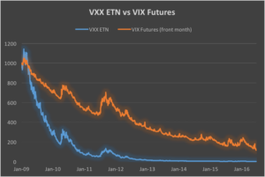
This phenomenon gives rise to opportunities for “carry” strategies, wherein a long volatility product such as VXX is sold in expectation that it will decline in value over time. Such strategies work well during periods when volatility futures are in contango, i.e. when the longer dated futures contracts have higher prices than shorter dated futures contracts and the spot VIX Index, which is typically the case around 70% of the time. An analogous strategy in the fixed income world is known as “riding down the yield curve”. When yield curves are upward sloping, a fixed income investor can buy a higher-yielding bill or bond in the expectation that the yield will decline, and the price rise, as the security approaches maturity. Quantitative easing put paid to that widely utilized technique, but analogous strategies in currency and volatility markets continue to perform well.
The challenge for any carry strategy is what happens when the curve inverts, as futures move into backwardation, often giving rise to precipitous losses. A variety of hedging schemes have been devised that are designed to mitigate the risk. For example, one well-known carry strategy in VIX futures entails selling the front month contract and hedging with a short position in an appropriate number of E-Mini S&P 500 futures contracts. In this case the hedge is imperfect, leaving the investor the task of managing a significant basis risk.

The chart of the compounded value of the VXX and VIX futures contract suggests another approach. While both securities decline in value over time, the fall in the value of the VXX ETN is substantially greater than that of the front month futures contract. The basic idea, therefore, is a relative value trade, in which we purchase VIX futures, the better performing of the pair, while selling the underperforming VXX. Since the value of the VXX is determined by the value of the front two months VIX futures contracts, the hedge, while imperfect, is likely to entail less basis risk than is the case for the VIX-ES futures strategy.
Another way to think about the trade is this: by combining a short position in VXX with a long position in the front-month futures, we are in effect creating a residual exposure in the value of the second month VIX futures contract relative to the first. So this is a strategy in which we are looking to capture volatility carry, not at the front of the curve, but between the first and second month futures maturities. We are, in effect, riding down the belly of volatility curve.
The Relationship between VXX and VIX Futures
Let’s take a look at the relationship between the VXX and front month futures contract, which I will hereafter refer to simply as VX. A simple linear regression analysis of VXX against VX is summarized in the tables below, and confirms two features of their relationship.
Firstly there is a strong, statistically significant relationship between the two (with an R-square of 75% ) – indeed, given that the value of the VXX is in part determined by VX, how could there not be?
Secondly, the intercept of the regression is negative and statistically significant. We can therefore conclude that the underperformance of the VXX relative to the VX is not just a matter of optics, but is a statistically reliable phenomenon. So the basic idea of selling the VXX against VX is sound, at least in the statistical sense.

Constructing the Initial Portfolio
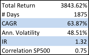
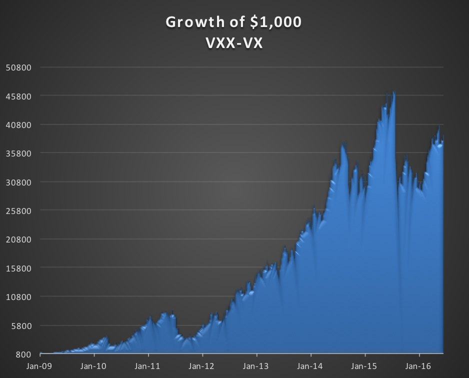
In constructing our theoretical portfolio, I am going to gloss over some important technical issues about how to construct the optimal hedge and simply assert that the best one can do is apply a beta of around 1.2, to produce the following outcome:
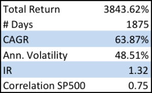

While broadly positive, with an information ratio of 1.32, the strategy performance is a little discouraging, on several levels. Firstly, the annual volatility, at over 48%, is uncomfortably high. Secondly, the strategy experiences very substantial drawdowns at times when the volatility curve inverts, such as in August 2015 and January 2016. Finally, the strategy is very highly correlated with the S&P500 index, which may be an important consideration for investors looking for ways to diversity their stock portfolio risk.
Exploiting Calendar Effects
We will address these issues in short order. Firstly, however, I want to draw attention to an interesting calendar effect in the strategy (using a simple pivot table analysis).

As you can see from the table above, the strategy returns in the last few days of the calendar month tend to be significantly below zero.
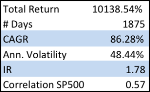
The cause of the phenomenon has to do with the way the VXX is constructed, but the important point here is that, in principle, we can utilize this effect to our advantage, by reversing the portfolio holdings around the end of the month. This simple technique produces a significant improvement in strategy returns, while lowering the correlation:
Reducing Portfolio Risk and Correlation
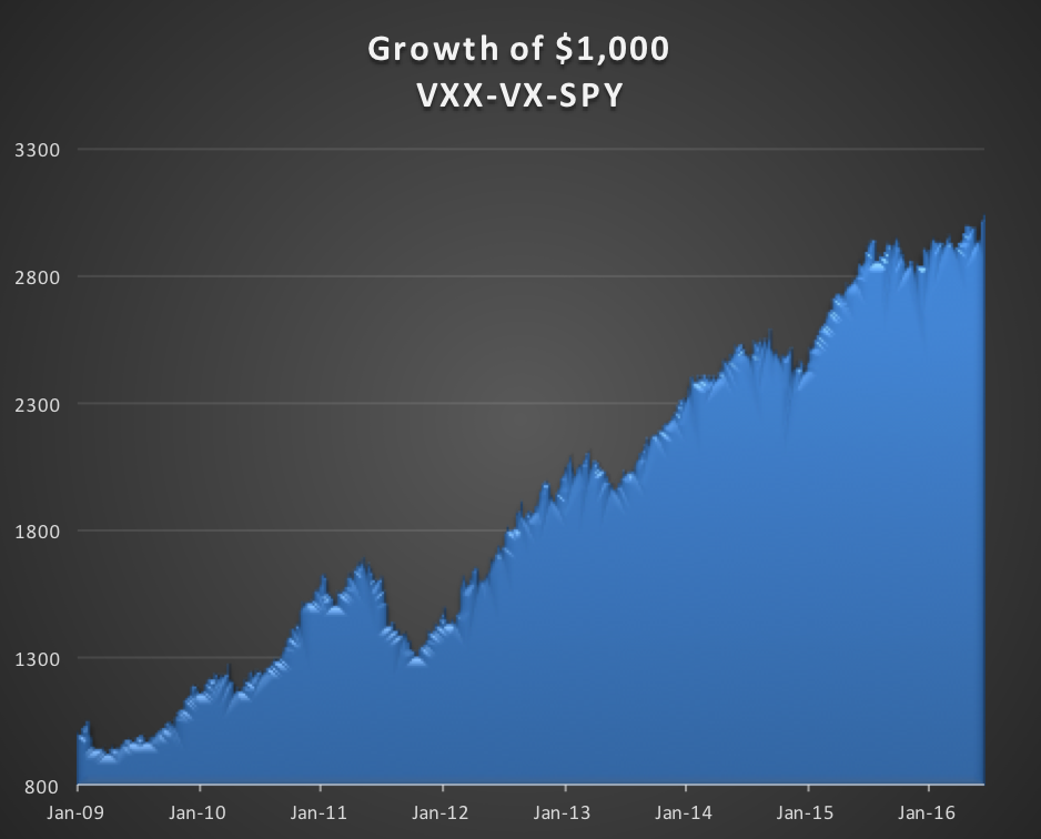
We can now address the issue of the residual high level of strategy volatility, while simultaneously reducing the strategy correlation to a much lower level. We can do this in a straightforward way by adding a third asset, the SPDR S&P 500 ETF Trust (NYSEArca:SPY), in which we will hold a short position, to exploit the negative correlation of the original portfolio.
We then adjust the portfolio weights to maximize the risk-adjusted returns, subject to limits on the maximum portfolio volatility and correlation. For example, setting a limit of 10% for both volatility and correlation, we achieve the following result (with weights -0.37 0.27 -0.65 for VXX, VX and SPY respectively):
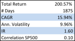

Compared to the original portfolio, the new portfolio’s performance is much more benign during the critical period from Q2-2015 to Q1-2016 and while there remain several significant drawdown periods, notably in 2011, overall the strategy is now approaching an investable proposition, with an information ratio of 1.6 and annual volatility of 9.96% and correlation of 0.1.
Other configurations are possible, of course, and the risk-adjusted performance can be improved, depending on the investor’s risk preferences.
Portfolio Rebalancing
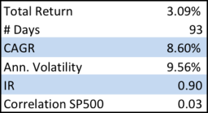
There is an element of curve-fitting in the research process as described so far, in as much as we are using all of the available data to July 2016 to construct a portfolio with the desired characteristics. In practice, of course, we will be required to rebalance the portfolio on a periodic basis, re-estimating the optimal portfolio weights as new data comes in. By way of illustration, the portfolio was re-estimated using in-sample data to the end of Feb, 2016, producing out-of-sample results during the period from March to July 2016, as follows:
A detailed examination of the generic problem of how frequently to rebalance the portfolio is beyond the scope of this article and I leave it to interested analysts to perform the research for themselves.
Practical Considerations
In order to implement the theoretical strategy described above there are several important practical steps that need to be considered.
- It is not immediately apparent how the weights should be applied to a portfolio comprising both ETNs and futures. In practice the best approach is to re-estimate the portfolio using a regression relationship expressed in $-value terms, rather than in percentages, in order to establish the quantity of VXX and SPY stock to be sold per single VX futures contract.
- Reversing the portfolio holdings in the last few days of the month will add significantly to transaction costs, especially for the position in VX futures, for which the minimum tick size is $50. It is important to factor realistic estimates of transaction costs into the assessment of the strategy performance overall and specifically with respect to month-end reversals.
- The strategy assumed the availability of VXX and SPY to short, which occasionally can be a problem. It’s not such a big deal if you are maintaining a long-term short position, but flipping the position around over a few ays at the end of the month might be problematic, from time to time.
- Also, we should take account of stock loan financing costs, which run to around 2.9% and 0.42% annually for VXX and SPY, respectively. These rates can vary with market conditions and stock availability, of course.
- It is highly likely that other ETFs/ETNs could profitably be added to the mix in order to further reduce strategy volatility and improve risk-adjusted returns. Likely candidates could include, for example, the Direxion Daily 20+ Yr Trsy Bull 3X ETF (NYSEArca:TMF).
- We have already mentioned the important issue of portfolio rebalancing. There is an argument for rebalancing more frequently to take advantage of the latest market data; on the other hand, too-frequent changes in the portfolio composition can undermine portfolio robustness, increase volatility and incur higher transaction costs. The question of how frequently to rebalance the portfolio is an important one that requires further testing to determine the optimal rebalancing frequency.
Conclusion
We have described the process of constructing a volatility carry strategy based on the relative value of the VXX ETN vs the front-month contract in VIX futures. By combining a portfolio comprising short positions in VXX and SPY with a long position in VIX futures, the investor can, in principle achieve risk-adjusted returns corresponding to an information ratio of around 1.6, or more. It is thought likely that further improvements in portfolio performance can be achieved by adding other ETFs to the portfolio mix.