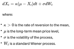
Consider a financial asset whose price, Xt, follows a mean-reverting stochastic process. A common model for mean reversion is the Ornstein-Uhlenbeck (OU) process, defined by the stochastic differential equation (SDE):
Objective
The trader aims to maximize the expected cumulative profit from trading this asset over a finite horizon, subject to transaction costs. The trader’s control is the rate of buying or selling the asset, denoted by ut, at time t.
Hamilton-Jacobi-Bellman (HJB) Equation
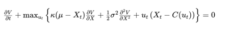
To find the optimal trading strategy, we frame this as a stochastic control problem. The value function,V(t,Xt), represents the maximum expected profit from time t to the end of the trading horizon, given the current price level Xt. The HJB equation for this problem is:
where C(ut) represents the cost of trading, which can depend on the rate of trading ut. The term ut(Xt−C(ut)) captures the profit from trading, adjusted for transaction costs.
Solution Approach
Boundary and Terminal Conditions: Specify terminal conditions for V(T,XT), where T is the end of the trading horizon, and boundary conditions for V(t,Xt) based on the problem setup.
Solve the HJB Equation: The solution involves finding the function V(t,Xt) and the control policy ut∗ that maximizes the HJB equation. This typically requires numerical methods, especially for complex cost functions or when closed-form solutions are not feasible.
Interpret the Optimal Policy: The optimal control ut∗ derived from solving the HJB equation indicates the optimal rate of trading (buying or selling) at any time t and price level Xt, considering the mean-reverting nature of the price and the impact of transaction costs.
Key Insights
No-Trade Zones: The presence of transaction costs often leads to the creation of no-trade zones in the optimal policy, where the expected benefit from trading does not outweigh the costs.
Mean-Reversion Exploitation: The optimal strategy exploits mean reversion by adjusting the trading rate based on the deviation of the current price from the mean level, μ.
The Lipton & Lopez de Marcos Paper
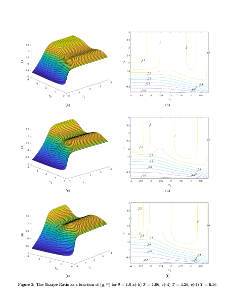
“A Closed-form Solution for Optimal Mean-reverting Trading Strategies” contributes significantly to the literature on optimal trading strategies for mean-reverting instruments. The paper focuses on deriving optimal trading strategies that maximize the Sharpe Ratio by solving the Hamilton-Jacobi-Bellman equation associated with the problem. It outlines a method that relies on solving a Fredholm integral equation to determine the optimal trading levels, taking into account transaction costs.
The paper begins by discussing the relevance of mean-reverting trading strategies across various markets, particularly emphasizing the energy market’s suitability for such strategies. It acknowledges the practical challenges and limitations of previous analytical results, mainly asymptotic and applicable to perpetual trading strategies, and highlights the novelty of addressing finite maturity strategies.
A key contribution of the paper is the development of an explicit formula for the Sharpe ratio in terms of stop-loss and take-profit levels, which allows traders to deploy tactical execution algorithms for optimal strategy performance under different market regimes. The methodology involves calibrating the Ornstein-Uhlenbeck process to market prices and optimizing the Sharpe ratio with respect to the defined levels. The authors present numerical results that illustrate the Sharpe ratio as a function of these levels for various parameters and discuss the implications of their findings for liquidity providers and statistical arbitrage traders.
The paper also reviews traditional approaches to similar problems, including the use of renewal theory and linear transaction costs, and compares these with its analytical framework. It concludes that its method provides a valuable tool for liquidity providers and traders to optimally execute their strategies, with practical applications beyond theoretical interest.
The authors use the path integral method to understand the behavior of their solutions, providing an alternative treatment to linear transaction costs that results in a determination of critical boundaries for trading. This approach is distinct in its use of direct solving methods for the Fredholm equation and adjusting the trading thresholds through a numerical method until a matching condition is met.
This research not only advances the understanding of optimal trading rules for mean-reverting strategies but also offers practical guidance for traders and liquidity providers in implementing these strategies effectively.
Market timing has a very bad press and for good reason: the inherent randomness of markets makes reliable forecasting virtually impossible. So why even bother to write about it? The answer is, because market timing has been mischaracterized and misunderstood. It isn’t about forecasting. If fact, with notable exceptions, most of trading isn’t about forecasting. It’s about conditional expectations.
Conditional expectations refer to the expected value of a random variable (such as future stock returns) given certain known information or conditions.
In the context of trading and market timing, it means that rather than attempting to forecast absolute price levels, we base our expectations for future returns on current observable market conditions.
For example, let’s say historical data shows that when the market has declined a certain percentage from its recent highs (condition), forward returns over the next several days tend to be positive on average (expectation). A trading strategy could use this information to buy the dip when that condition is met, not because it is predicting that the market will rally, but because history suggests a favorable risk/reward ratio for that trade under those specific circumstances.
The key insight is that by focusing on conditional expectations, we don’t need to make absolute predictions about where the market is heading. We simply assess whether the present conditions have historically been associated with positive expected returns, and use that probabilistic edge to inform our trading decisions.
This is a more nuanced and realistic approach than binary forecasting, as it acknowledges the inherent uncertainty of markets while still allowing us to make intelligent, data-driven decisions. By aligning our trades with conditional expectations, we can put the odds in our favor without needing a crystal ball.
So, when a market timing algorithm suggests buying the market, it isn’t making a forecast about what the market is going to do next. Rather, what it is saying is, if the market behaves like this then, on past experience, the following trade is likely to be profitable. That is a very different thing from forecasting the market.
A good example of a simple market-timing algorithm is “buying the dips”. It’s so simple that you don’t need a computer algorithm to do it. But a computer algorithm helps by determining what comprises a dip and the level at which profits should be taken.
An Effective Market Timing Strategy
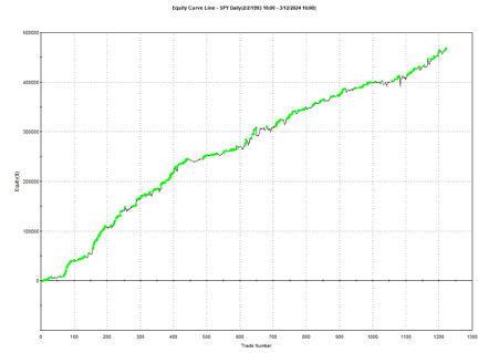
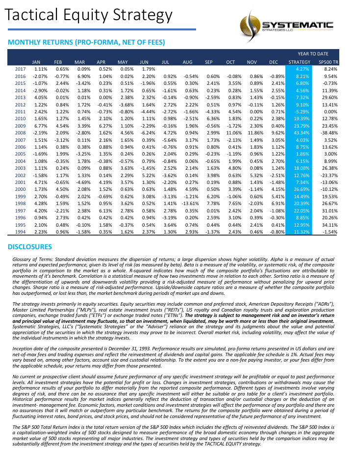
One of my favorites market timing strategies is the following algorithm, which I originally developed to trade the SPY ETF. The equity curve from inception of the ETF in 1993 looks like this:
The algorithm combines a few simple technical indicators to determine what constitutes a dip and the level at which profits should be taken. The entry and exit orders are also very straightforward, buying and selling at the market open, which can be achieved by participating in the opening auction. This is very convenient: a signal is generated after the close on day 1 and is then executed as a MOA (market opening auction) order in the opening auction on day 2. The opening auction is by no means the most liquid period of the trading session, but in an ETF like SPY the volumes are such that the market impact is likely to be negligible for the great majority of investors. This is not something you would attempt to do in an illiquid small-cap stock, however, where entries and exits are more reliably handled using a VWAP algorithm; but for any liquid ETF or large-cap stock the opening auction will typically be fine.
Adapting the Strategy to Other Assets and Markets
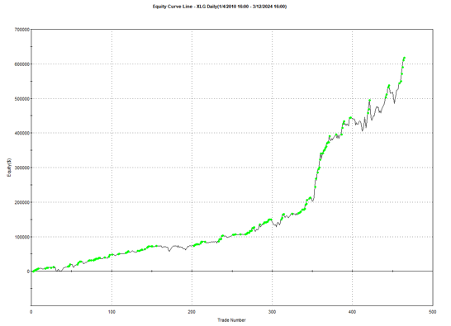
Another aspect that gives me confidence in the algorithm is that it generalizes well to other assets and even other markets. Here, for example, is the equity curve for the exact same algorithm implemented in the XLG ETF in the period from 2010:
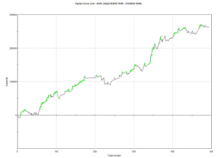
And here is the equity curve for the same strategy (with the same parameters) in AAPL, over the same period:
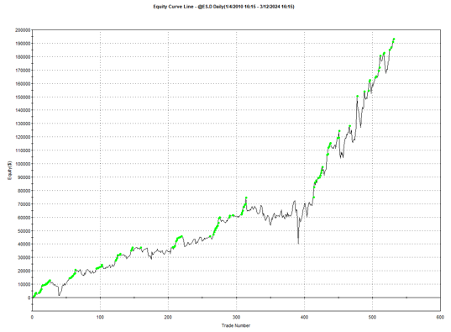
Remarkably, the strategy also works in E-mini futures too, which is highly unusual: typically the market dynamics of the futures market are so different from the spot market that strategies don’t transfer well. But in this case, it simply works:
Understanding Why the Strategy Works
The reason the strategy is effective is due to the upward drift in equities and related derivatives. If you tried to apply a similar strategy to energy or currency markets, it would fail. The strategy’s “secret sauce” is the combination of indicators it uses to determine the short-term low in the ETF that constitutes a good buying opportunity, and then figure out the right level at which to sell.
Does the algorithm always work? If by that you mean “is every trade profitable?” the answer is no. Around 61% of trades are profitable, so there are many instances where trades are closed at a loss. But the net impact of using the market-timing algorithm is very positive, when compared to the buy-and-hold benchmark, as we shall see shortly.
Because the underlying thesis is so simple (i.e. equity markets have positive drift), we can say something about the long-term prospects for the strategy. Equity markets haven’t changed their fundamental tendency to appreciate over the 31-year period from inception of the SPY ETF in 1993, which is why the strategy has performed well throughout that time. Could one envisage market conditions in which the strategy will perform poorly? Yes – any prolonged period of flat to downward trending prices in equities will result in poor performance. But we haven’t seen those conditions since the early 1970’s and, arguably, they are unlikely to return, since the fundamental change brought about by abandonment of the gold standard in 1973.
The abandonment of the gold standard and the subsequent shift to fiat currencies has given central banks, particularly the U.S. Federal Reserve, unprecedented power to expand the money supply and support asset prices during times of crisis. This ‘Fed Put’ has been a major factor underpinning the multi-decade bull market in stocks.
In addition, the increasing dominance of the U.S. as the world’s primary economic and military superpower since the end of the Cold War has made U.S. financial assets a uniquely attractive destination for global capital, creating sustained demand for U.S. equities.
Technological innovation, particularly with respect to the internet and advances in computing, has also unleashed a wave of productivity and wealth creation that has disproportionately benefited the corporate sector and equity holders. This trend shows no signs of abating and may even be accelerating with the advent of artificial intelligence.
While risks certainly remain and occasional cyclical bear markets are inevitable, the combination of accommodative monetary policy, the U.S.’s global hegemony, and technological progress create a powerful set of economic forces that are likely to continue propelling equity prices higher over the long-term, albeit with significant volatility along the way.Strategy Performance in Bear Markets
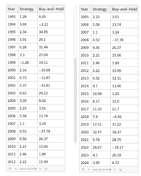
Note that the conditions I am referring to are something unlike anything we have seen in the last 50 years, not just a (serious) market pullback. If we look at the returns in the period from 2000-2002, for example, we see that the strategy held up very well, out-performing the benchmark by 54% over the three-year period of the market crash. Likewise, in 2008 credit crisis, the strategy was able to eke out a small gain, beating the benchmark by over 38%. In fact, the strategy is positive in all but one of the 31 years from inception.
Comparing Performance to Buy-and-Hold
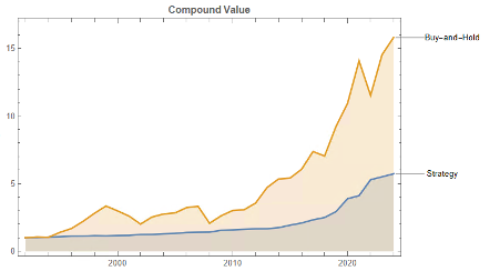
Let’s take a look at the compound returns from the strategy vs. the buy-and-hold benchmark:
At first sight, it appears that the benchmark significantly out-performs the strategy, albeit suffering from much larger drawdowns. But that doesn’t give an accurate picture of relative performance. To see why, let’s look at the overall performance characteristics:
Now we see that, while the strategy CAGR is 3.50% below the buy-and-hold return, its annual volatility is less than half that of the benchmark, giving the strategy a superior Sharpe Ratio.
Leveraging the Strategy to Enhance Risk-Adjusted Returns
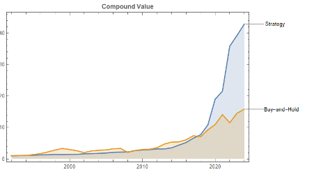
To make a valid comparison between the strategy and its benchmark we therefore need to equalize the annual volatility of both, and we can achieve this by leveraging the strategy by a factor of approximately 2.32. When we do that, we obtain the following results:
Now that the strategy and benchmark volatilities have been approximately equalized through leverage, we see that the strategy substantially outperforms buy-and-hold by around 355 basis points per year and with far smaller drawdowns.
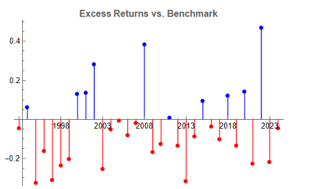
In general, we see that the strategy outperformed the benchmark in fewer than 50% of annual periods since 1993. However, the size of the outperformance in years when it beat the benchmark was frequently very substantial:
Conclusion
Market timing can work. To understand why, we need to stop thinking in terms of forecasting and think instead about conditional returns. When we do that, we arrive at the insight that market timing works because it relies on the positive drift in equity markets, which has been one of the central features of that market over the last 50 years and is likely to remain so in the foreseeable future. We have confidence in that prediction, because we understand the economic factors that have continued to drive the upward drift in equities over the last half-century.
After that, it is simply a question of the mechanics – how to time the entries and exits. This article describes just one approach amongst a great number of possibilities.
One of the many benefits of market timing is that it has a tendency to side-step the worst market conditions and can produce positive returns even in the most hostile environments: periods such as 2000-2002 and 2008, for example, as we have seen.
Finally, don’t forget that, as we are sitting out of the market approximately 40% of the time our overall risk is much lower – less than half that of the benchmark. So, we can afford to leverage our positions without taking on more overall risk than when we buy and hold. This clearly demonstrates the ability of the strategy to produce higher rates of risk-adjusted return.
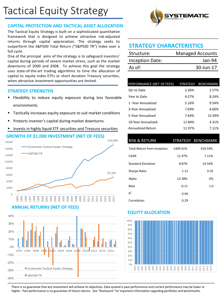
We have created a long-only equity strategy that aims to beat the S&P 500 total return benchmark by using tactical allocation algorithms to invest in equity ETFs. One of the principal goals of the strategy is to protect investors’ capital during periods of severe market stress such as in the downturns of 2000 and 2008. The strategy times the allocation of capital to equity ETFs or short-duration Treasury securities when investment opportunities are limited.
Systematic Strategies is a hedge fund rather than an RIA, so we have no plans to offer the product to the public. However, we are currently holding exploratory discussions with Registered Investment Advisors about how the strategy might be made available to their clients.
For more background, see this post on Seeking Alpha: http://tiny.cc/ba3kny
Around a quarter of a century ago I wrote a paper entitled “Equity Convexity” which – to my disappointment – was rejected as incomprehensible by the finance professor who reviewed it. But perhaps I should not have expected more: novel theories are rarely well received first time around. I remain convinced the idea has merit and may perhaps revisit it in these pages at some point in future. For now, I would like to discuss a related, but simpler concept: beta convexity. As far as I am aware this, too, is new. At least, while I find it unlikely that it has not already been considered, I am not aware of any reference to it in the literature.
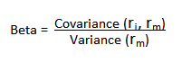
We begin by reviewing the elementary concept of an asset beta, which is the covariance of the return of an asset with the return of the benchmark market index, divided by the variance of the return of the benchmark over a certain period:
Asset betas typically exhibit time dependency and there are numerous methods that can be used to model this feature, including, for instance, the Kalman Filter:
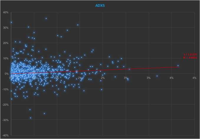
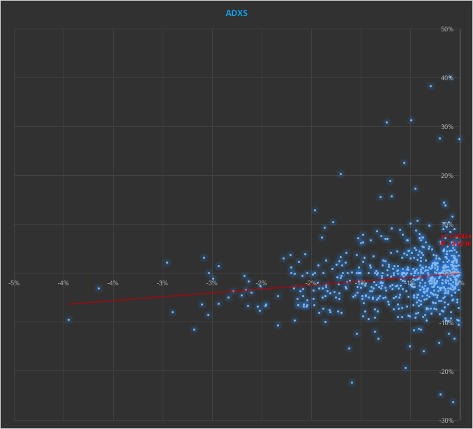
In the context discussed here we set such matters to one side. Instead of considering how an asset beta may vary over time, we look into how it might change depending on the direction of the benchmark index. To take an example, let’s consider the stock Advaxis, Inc. (Nasdaq: ADXS). In the charts below we examine the relationship between the daily stock returns and the returns in the benchmark Russell 3000 Index when the latter are positive and negative.
The charts indicate that the stock beta tends to be higher during down periods in the benchmark index than during periods when the benchmark return is positive. This can happen for two reasons: either the correlation between the asset and the index rises, or the volatility of the asset increases, (or perhaps both) when the overall market declines. In fact, over the period from Jan 2012 to May 2017, the overall stock beta was 1.31, but the up-beta was only 0.44 while the down-beta was 1.53. This is quite a marked difference and regardless of whether the change in beta arises from a change in the correlation or in the stock volatility, it could have a significant impact on the optimal weighting for this stock in an equity portfolio.
Ideally, what we would prefer to see is very little dependence in the relationship between the asset beta and the sign of the underlying benchmark. One way to quantify such dependency is with what I have called Beta Convexity:
Beta Convexity = (Up-Beta – Down-Beta) ^2
A stock with a stable beta, i.e. one for which the difference between the up-beta and down-beta is negligibly small, will have a beta-convexity of zero. One the other hand, a stock that shows instability in its beta relationship with the benchmark will tend to have relatively large beta convexity.
Index Replication using a Minimum Beta-Convexity Portfolio
One way to apply this concept it to use it as a means of stock selection. Regardless of whether a stock’s overall beta is large or small, ideally we want its dependency to be as close to zero as possible, i.e. with near-zero beta-convexity. This is likely to produce greater stability in the composition of the optimal portfolio and eliminate unnecessary and undesirable excess volatility in portfolio returns by reducing nonlinearities in the relationship between the portfolio and benchmark returns.
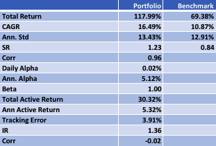
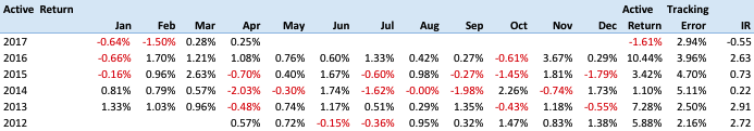
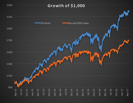
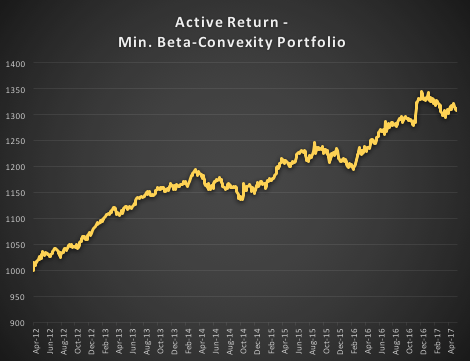
In the following illustration we construct a stock portfolio by choosing the 500 constituents of the benchmark Russell 3000 index that have the lowest beta convexity during the previous 90-day period, rebalancing every quarter (hence all of the results are out-of-sample). The minimum beta-convexity portfolio outperforms the benchmark by a total of 48.6% over the period from Jan 2012-May 2017, with an annual active return of 5.32% and Information Ratio of 1.36. The portfolio tracking error is perhaps rather too large at 3.91%, but perhaps can be further reduced with the inclusion of additional stocks.
Conclusion: Beta Convexity as a New Factor
Beta convexity is a new concept that appears to have a useful role to play in identifying stocks that have stable long term dependency on the benchmark index and constructing index tracking portfolios capable of generating appreciable active returns.
The outperformance of the minimum-convexity portfolio is not the result of a momentum effect, or a systematic bias in the selection of high or low beta stocks. The selection of the 500 lowest beta-convexity stocks in each period is somewhat arbitrary, but illustrates that the approach can scale to a size sufficient to deploy hundreds of millions of dollars of investment capital, or more. A more sensible scheme might be, for example, to select a variable number of stocks based on a predefined tolerance limit on beta-convexity.
Obvious steps from here include experimenting with alternative weighting schemes such as value or beta convexity weighting and further refining the stock selection procedure to reduce the portfolio tracking error.
Further useful applications of the concept are likely to be found in the design of equity long/short and market neural strategies. These I shall leave the reader to explore for now, but I will perhaps return to the topic in a future post.