
“The first rule of investing isn’t ‘Don’t lose money.’ It’s ‘Recognize when the rules are changing.'”
UPDATE: MAY 1 2025
The February 2025 European semiconductor export restrictions sent markets into a two-day tailspin, wiping $1.3 trillion from global equities. For most investors, it was another stomach-churning reminder of how traditional portfolios falter when geopolitics overwhelms fundamentals.
But for a growing cohort of forward-thinking portfolio managers, it was validation. Their Strategic Scenario Portfolios—deliberately constructed to thrive during specific geopolitical events—delivered positive returns amid the chaos.
I’m not talking about theoretical models. I’m talking about real money, real returns, and a methodology you can implement right now.
What Exactly Is a Strategic Scenario Portfolio?
A Strategic Scenario Portfolio (SSP) is an investment allocation designed to perform robustly during specific high-impact events—like trade wars, sanctions, regional conflicts, or supply chain disruptions.
Unlike conventional approaches that react to crises, SSPs anticipate them. They’re narrative-driven, built around specific, plausible scenarios that could reshape markets. They’re thematically concentrated, focusing on sectors positioned to benefit from that scenario rather than broad diversification. They maintain asymmetric balance, incorporating both downside protection and upside potential. And perhaps most importantly, they’re ready for deployment before markets fully price in the scenario.
Think of SSPs as portfolio “insurance policies” that also have the potential to deliver substantial alpha.
“Why didn’t I know about this before now?” SSPs aren’t new—institutional investors have quietly used similar approaches for decades. What’s new is systematizing this approach for broader application.
Real-World Proof: Two Case Studies That Speak for Themselves
Case Study #1: The 2018-2019 US-China Trade War
When trade tensions escalated in 2018, we constructed the “USChinaTradeWar2018” portfolio with a straightforward mandate: protect capital while capitalizing on trade-induced dislocations.
The portfolio allocated 25% to SPDR Gold Shares (GLD) as a core risk-off hedge. Another 20% went to Consumer Staples (VDC) for defensive positioning, while 15% was invested in Utilities (XLU) for stable returns and low volatility. The remaining 40% was distributed equally among Walmart (WMT), Newmont Mining (NEM), Procter & Gamble (PG), and Industrials (XLI), creating a balanced mix of defensive positioning with selective tactical exposure.
The results were remarkable. From May 2018 to December 2019, this portfolio delivered a total return of 30.2%, substantially outperforming the S&P 500’s 22.0%. More impressive than the returns, however, was the risk profile. The portfolio achieved a Sharpe ratio of 1.8 (compared to the S&P 500’s 0.6), demonstrating superior risk-adjusted performance. Its maximum drawdown was a mere 2.2%, while the S&P 500 experienced a 14.0% drawdown during the same period. With a beta of just 0.26 and alpha of 11.7%, this portfolio demonstrated precisely what SSPs are designed to deliver: outperformance with dramatically reduced correlation to broader market movements.
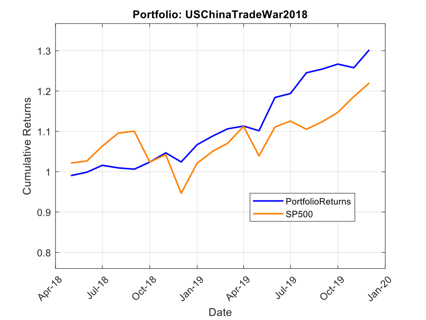
Note: Past performance is not indicative of future results. Performance calculated using total return with dividends reinvested, compared against S&P 500 total return.
Case Study #2: The 2025 Tariff War Portfolio
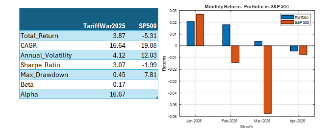
Fast forward to January 2025. With new tariffs threatening global trade, we developed the “TariffWar2025” portfolio using a similar strategic framework but adapted to the current environment.
The core of the portfolio (50%) established a defensive foundation across Utilities (XLU), Consumer Staples (XLP), Healthcare (XLV), and Gold (GLD). We allocated 20% toward domestic industrial strength through Industrials (XLI) and Energy (XLE) to capture reshoring benefits and energy independence trends. Another 20% targeted strategic positioning with Lockheed Martin (LMT) benefiting from increased defense spending and Cisco (CSCO) offering exposure to domestic technology infrastructure with limited Chinese supply chain dependencies. The remaining 10% created balanced treasury exposure across long-term (TLT) and short-term (VGSH) treasuries to hedge against both economic slowdown and rising rates.
The results through Q1 2025 have been equally impressive. While the S&P 500 declined 4.6%, the TariffWar2025 portfolio generated a positive 4.3% return. Its Sharpe ratio of 8.4 indicates exceptional risk-adjusted performance, and remarkably, the portfolio experienced zero drawdown during a period when the S&P 500 fell by as much as 7.1%. With a beta of 0.20 and alpha of 31.9%, the portfolio again demonstrated the power of scenario-based investing in navigating geopolitical turbulence.
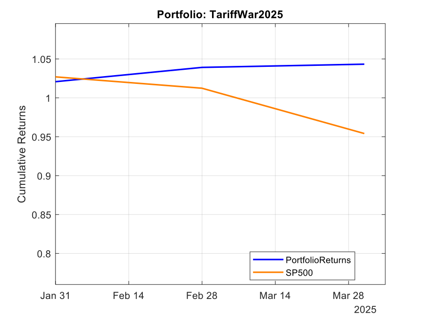
Note: Past performance is not indicative of future results. Performance calculated using total return with dividends reinvested, compared against S&P 500 total return.
Why Traditional Portfolios Fail When You Need Them Most
Traditional portfolio construction relies heavily on assumptions that often crumble during times of geopolitical stress. Historical correlations, which form the backbone of most diversification strategies, routinely break during crises. Mean-variance optimization, a staple of modern portfolio theory, falters dramatically when markets exhibit non-normal distributions, which is precisely what happens during geopolitical events. And the broad diversification that works so well in normal times often converges in stressed markets, leaving investors exposed just when protection is most needed.
When markets fracture along geopolitical lines, these assumptions collapse spectacularly. Consider the March 2023 banking crisis: correlations between tech stocks and regional banks—historically near zero—suddenly jumped to 0.75. Or recall how in 2022, both stocks AND bonds declined simultaneously, shattering the foundation of 60/40 portfolios.
What geopolitical scenario concerns you most right now, and how is your portfolio positioned for it? This question reveals the central value proposition of Strategic Scenario Portfolios.
Building Your Own Strategic Scenario Portfolio: A Framework for Success
You don’t need a quant team to implement this approach. The framework begins with defining a clear scenario. Rather than vague concerns about “volatility” or “recession,” an effective SSP requires a specific narrative. For example: “Europe imposes carbon border taxes, triggering retaliatory measures from major trading partners.”
From this narrative foundation, you can map the macro implications. Which regions would face the greatest impact? What sectors would benefit or suffer? How might interest rates, currencies, and commodities respond? This mapping process translates your scenario into investment implications.
The next step involves identifying asymmetric opportunities—situations where the market is underpricing both risks and potential benefits related to your scenario. These asymmetries create the potential for alpha generation within your protective framework.
Structure becomes critical at this stage. A typical SSP balances defensive positions (usually 60-75% of the allocation) with opportunity capture (25-40%). This balance ensures capital preservation while maintaining upside potential if your scenario unfolds as anticipated.
Finally, establish monitoring criteria. Define what developments would strengthen or weaken your scenario’s probability, and set clear guidelines for when to increase exposure, reduce positions, or exit entirely.
For those new to this approach, start with a small allocation—perhaps 5-10% of your portfolio—as a satellite to your core holdings. As your confidence or the scenario probability increases, you can scale up exposure accordingly.
Common Questions About Strategic Scenario Portfolios
“Isn’t this just market timing in disguise?” This question arises frequently, but the distinction is important. Market timing attempts to predict overall market movements—when the market will rise or fall. SSPs are fundamentally different. They’re about identifying specific scenarios and their sectoral impacts, regardless of broad market direction. The focus is on relative performance within a defined context, not on predicting market tops and bottoms.
“How do I know when to exit an SSP position?” The key is defining exit criteria in advance. This might include scenario resolution (like a trade agreement being signed), time limits (reviewing the position after a predefined period), or performance thresholds (taking profits or cutting losses at certain levels). Clear exit strategies prevent emotional decision-making when markets become volatile.
“Do SSPs work in all market environments?” This question reveals a misconception about their purpose. SSPs aren’t designed to outperform in all environments. They’re specifically built to excel during their target scenarios, while potentially underperforming in others. That’s why they work best as tactical overlays to core portfolios, rather than as stand-alone investment approaches.
“How many scenarios should I plan for simultaneously?” Start with one or two high-probability, high-impact scenarios. Too many simultaneous SSPs can dilute your strategic focus and create unintended exposures. As you gain comfort with the approach, you can expand your scenario coverage while maintaining portfolio coherence.
Tools for the Forward-Thinking Investor
Implementing SSPs effectively requires both qualitative and quantitative tools. Systems like the Equities Entity Store for MATLAB provide institutional-grade capabilities for modeling multi-asset correlations across different regimes. They enable stress-testing portfolios against specific geopolitical scenarios, optimizing allocations based on scenario probabilities, and tracking exposures to factors that become relevant primarily in crisis periods.
These tools help translate scenario narratives into precise portfolio allocations with targeted risk exposures. While sophisticated analytics enhance the process, the core methodology remains accessible even to investors without advanced quantitative resources.
The Path Forward in a Fractured World
The investment landscape of 2025 is being shaped by forces that traditional models struggle to capture. Deglobalization and reshoring are restructuring supply chains and changing regional economic dependencies. Resource nationalism and energy security concerns are creating new commodity dynamics. Strategic competition between major powers is manifesting in investment restrictions, export controls, and targeted sanctions. Technology fragmentation along geopolitical lines is creating parallel innovation systems with different winners and losers.
In this environment, passive diversification is necessary but insufficient. Strategic Scenario Portfolios provide a disciplined framework for navigating these challenges, protecting capital, and potentially generating significant alpha when markets are most volatile.
The question isn’t whether geopolitical disruptions will continue—they will. The question is whether your portfolio is deliberately designed to withstand them.
Next Steps: Getting Started With SSPs
The journey toward implementing Strategic Scenario Portfolios begins with identifying your most concerning scenario. What geopolitical or policy risk keeps you up at night? Is it escalation in the South China Sea? New climate regulations? Central bank digital currencies upending traditional banking?
Once you’ve identified your scenario, assess your current portfolio’s exposure. Would your existing allocations benefit, suffer, or remain neutral if this scenario materialized? This honest assessment often reveals vulnerabilities that weren’t apparent through traditional risk measures.
Design a prototype SSP focused on your scenario. Start small, perhaps with a paper portfolio that you can monitor without committing capital immediately. Track both the portfolio’s performance and developments related to your scenario, refining your approach as you gain insights.
For many investors, this process benefits from professional guidance. Complex scenario mapping requires a blend of geopolitical insight, economic analysis, and portfolio construction expertise that often exceeds the resources of individual investors or even smaller investment teams.
About the Author: Jonathan Kinlay, PhD is Principal Partner at Golden Bough Partners LLC, a quantitative proprietary trading firm, and managing partner of Intelligent Technologies. With experience as a finance professor at NYU Stern and Carnegie Mellon, he specializes in advanced portfolio construction, algorithmic trading systems, and quantitative risk management. His latest book, “Equity Analytics” (2024), explores modern approaches to market resilience. Jonathan works with select institutional clients and fintech ventures as a strategic advisor, helping them develop robust quantitative frameworks that deliver exceptional risk-adjusted returns. His proprietary trading systems have consistently achieved Sharpe ratios 2-3× industry benchmarks.
📬 Let’s Connect: Have you implemented scenario-based approaches in your investment process? What geopolitical risks are you positioning for? Share your thoughts in the comments or connect with me directly.
Disclaimer: This article is for informational purposes only and does not constitute investment advice. The performance figures presented are based on actual portfolios but may not be achievable for all investors. Always conduct your own research and consider your financial situation before making investment decisions.


