An extract from the chapter on pairs trading from my forthcoming book Equity Analytics
Pairs-Trading-1Robustness in Quantitative Research and Trading
What is Strategy Robustness? What is its relevance to Quantitative Research and Trading?
One of the most highly desired properties of any financial model or investment strategy, by investors and managers alike, is robustness. I would define robustness as the ability of the strategy to deliver a consistent results across a wide range of market conditions. It, of course, by no means the only desirable property – investing in Treasury bills is also a pretty robust strategy, although the returns are unlikely to set an investor’s pulse racing – but it does ensure that the investor, or manager, is unlikely to be on the receiving end of an ugly surprise when market conditions adjust.
Robustness is not the same thing as low volatility, which also tends to be a characteristic highly prized by many investors. A strategy may operate consistently, with low volatility in certain market conditions, but behave very differently in other. For instance, a delta-hedged short-volatility book containing exotic derivative positions. The point is that empirical researchers do not know the true data-generating process for the markets they are modeling. When specifying an empirical model they need to make arbitrary assumptions. An example is the common assumption that assets returns follow a Gaussian distribution. In fact, the empirical distribution of the great majority of asset process exhibit the characteristic of “fat tails”, which can result from the interplay between multiple market states with random transitions. See this post for details:
http://jonathankinlay.com/2014/05/a-quantitative-analysis-of-stationarity-and-fat-tails/
In statistical arbitrage, for example, quantitative researchers often make use of cointegration models to build pairs trading strategies. However the testing procedures used in current practice are not sufficient powerful to distinguish between cointegrated processes and those whose evolution just happens to correlate temporarily, resulting in the frequent breakdown in cointegrating relationships. For instance, see this post:
http://jonathankinlay.com/2017/06/statistical-arbitrage-breaks/
Modeling Assumptions are Often Wrong – and We Know It
We are, of course, not the first to suggest that empirical models are misspecified:
“All models are wrong, but some are useful” (Box 1976, Box and Draper 1987).
Martin Feldstein (1982: 829): “In practice all econometric specifications are necessarily false models.”
Luke Keele (2008: 1): “Statistical models are always simplifications, and even the most complicated model will be a pale imitation of reality.”
Peter Kennedy (2008: 71): “It is now generally acknowledged that econometric models are false and there is no hope, or pretense, that through them truth will be found.”
During the crash of 2008 quantitative Analysts and risk managers found out the hard way that the assumptions underpinning the copula models used to price and hedge credit derivative products were highly sensitive to market conditions. In other words, they were not robust. See this post for more on the application of copula theory in risk management:
http://jonathankinlay.com/2017/01/copulas-risk-management/
Robustness Testing in Quantitative Research and Trading
We interpret model misspecification as model uncertainty. Robustness tests analyze model uncertainty by comparing a baseline model to plausible alternative model specifications. Rather than trying to specify models correctly (an impossible task given causal complexity), researchers should test whether the results obtained by their baseline model, which is their best attempt of optimizing the specification of their empirical model, hold when they systematically replace the baseline model specification with plausible alternatives. This is the practice of robustness testing.
Robustness testing analyzes the uncertainty of models and tests whether estimated effects of interest are sensitive to changes in model specifications. The uncertainty about the baseline model’s estimated effect size shrinks if the robustness test model finds the same or similar point estimate with smaller standard errors, though with multiple robustness tests the uncertainty likely increases. The uncertainty about the baseline model’s estimated effect size increases of the robustness test model obtains different point estimates and/or gets larger standard errors. Either way, robustness tests can increase the validity of inferences.
Robustness testing replaces the scientific crowd by a systematic evaluation of model alternatives.
Robustness in Quantitative Research
In the literature, robustness has been defined in different ways:
- as same sign and significance (Leamer)
- as weighted average effect (Bayesian and Frequentist Model Averaging)
- as effect stability We define robustness as effect stability.
Parameter Stability and Properties of Robustness
Robustness is the share of the probability density distribution of the baseline model that falls within the 95-percent confidence interval of the baseline model. In formulaeic terms:
- Robustness is left-–right symmetric: identical positive and negative deviations of the robustness test compared to the baseline model give the same degree of robustness.
- If the standard error of the robustness test is smaller than the one from the baseline model, ρ converges to 1 as long as the difference in point estimates is negligible.
- For any given standard error of the robustness test, ρ is always and unambiguously smaller the larger the difference in point estimates.
- Differences in point estimates have a strong influence on ρ if the standard error of the robustness test is small but a small influence if the standard errors are large.
Robustness Testing in Four Steps
- Define the subjectively optimal specification for the data-generating process at hand. Call this model the baseline model.
- Identify assumptions made in the specification of the baseline model which are potentially arbitrary and that could be replaced with alternative plausible assumptions.
- Develop models that change one of the baseline model’s assumptions at a time. These alternatives are called robustness test models.
- Compare the estimated effects of each robustness test model to the baseline model and compute the estimated degree of robustness.
Model Variation Tests
Model variation tests change one or sometimes more model specification assumptions and replace with an alternative assumption, such as:
- change in set of regressors
- change in functional form
- change in operationalization
- change in sample (adding or subtracting cases)
Example: Functional Form Test
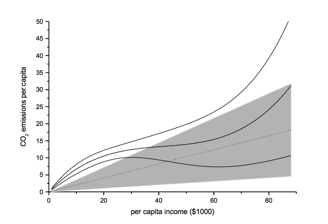
The functional form test examines the baseline model’s functional form assumption against a higher-order polynomial model. The two models should be nested to allow identical functional forms. As an example, we analyze the ‘environmental Kuznets curve’ prediction, which suggests the existence of an inverse u-shaped relation between per capita income and emissions.
Note: grey-shaded area represents confidence interval of baseline model
Another example of functional form testing is given in this review of Yield Curve Models:
http://jonathankinlay.com/2018/08/modeling-the-yield-curve/
Random Permutation Tests
Random permutation tests change specification assumptions repeatedly. Usually, researchers specify a model space and randomly and repeatedly select model from this model space. Examples:
- sensitivity tests (Leamer 1978)
- artificial measurement error (Plümper and Neumayer 2009)
- sample split – attribute aggregation (Traunmüller and Plümper 2017)
- multiple imputation (King et al. 2001)
We use Monte Carlo simulation to test the sensitivity of the performance of our Quantitative Equity strategy to changes in the price generation process and also in model parameters:
http://jonathankinlay.com/2017/04/new-longshort-equity/
Structured Permutation Tests
Structured permutation tests change a model assumption within a model space in a systematic way. Changes in the assumption are based on a rule, rather than random. Possibilities here include:
- sensitivity tests (Levine and Renelt)
- jackknife test
- partial demeaning test
Example: Jackknife Robustness Test
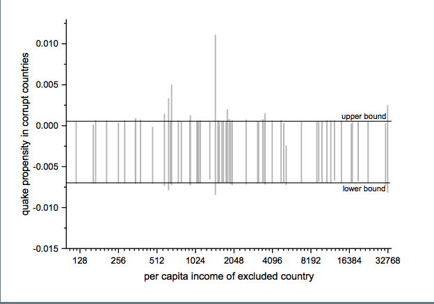
The jackknife robustness test is a structured permutation test that systematically excludes one or more observations from the estimation at a time until all observations have been excluded once. With a ‘group-wise jackknife’ robustness test, researchers systematically drop a set of cases that group together by satisfying a certain criterion – for example, countries within a certain per capita income range or all countries on a certain continent. In the example, we analyse the effect of earthquake propensity on quake mortality for countries with democratic governments, excluding one country at a time. We display the results using per capita income as information on the x-axes.
Upper and lower bound mark the confidence interval of the baseline model.
Robustness Limit Tests
Robustness limit tests provide a way of analyzing structured permutation tests. These tests ask how much a model specification has to change to render the effect of interest non-robust. Some examples of robustness limit testing approaches:
- unobserved omitted variables (Rosenbaum 1991)
- measurement error
- under- and overrepresentation
- omitted variable correlation
For an example of limit testing, see this post on a review of the Lognormal Mixture Model:
http://jonathankinlay.com/2018/08/the-lognormal-mixture-variance-model/
Summary on Robustness Testing
Robustness tests have become an integral part of research methodology. Robustness tests allow to study the influence of arbitrary specification assumptions on estimates. They can identify uncertainties that otherwise slip the attention of empirical researchers. Robustness tests offer the currently most promising answer to model uncertainty.
Metal Logic
Precious metals have been in free-fall for several years, as a consequence of the Fed’s actions to stimulate the economy that have also had the effect of goosing the equity and fixed income markets. All that changed towards the end of 2015, as the Fed moved to a tightening posture. So far, 2016 has been a banner year for metal, with spot prices for platinum, gold and silver up 26%, 28% and 44% respectively.
So what are the prospects for metals through the end of the year? We take a shot at predicting the outcome, from a quantitative perspective.
Source: Wolfram Alpha. Spot silver prices are scaled x100
Metals as Correlated Processes
One of the key characteristics of metals is the very high levels of price-correlation between them. Over the period under investigation, Jan 2012 to Aug 2016, the estimated correlation coefficients are as follows:
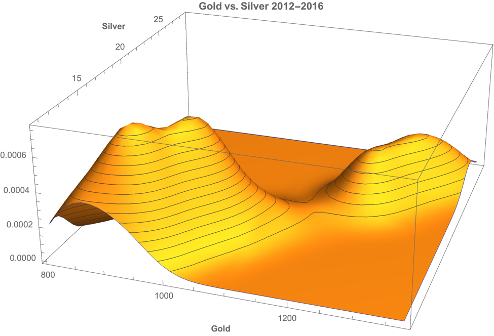
A plot of the join density of spot gold and silver prices indicates low- and high-price regimes in which the metals display similar levels of linear correlation.
Simple Metal Trading Models
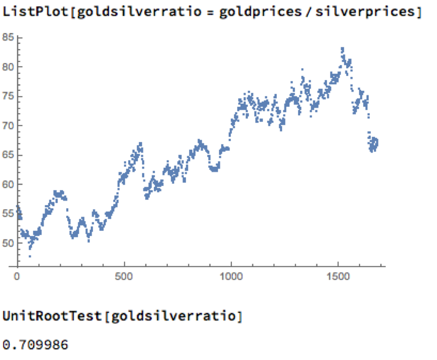
Levels of correlation that are consistently as high as this over extended periods of time are fairly unusual in financial markets and this presents a potential trading opportunity. One common approach is to use the ratios of metal prices as a trading signal. However, taking the ratio of gold to silver spot prices as an example, a plot of the series demonstrates that it is highly unstable and susceptible to long term trends.
A more formal statistical test fails to reject the null hypothesis of a unit root. In simple terms, this means we cannot reliably distinguish between the gold/silver price ratio and a random walk.
Along similar lines, we might consider the difference in log prices of the series. If this proved to be stationary then the log-price series would be cointegrated order 1 and we could build a standard pairs trading model to buy or sell the spread when prices become too far unaligned. However, we find once again that the log-price difference can wander arbitrarily far from its mean, and we are unable to reject the null hypothesis that the series contains a unit root.
Linear Models
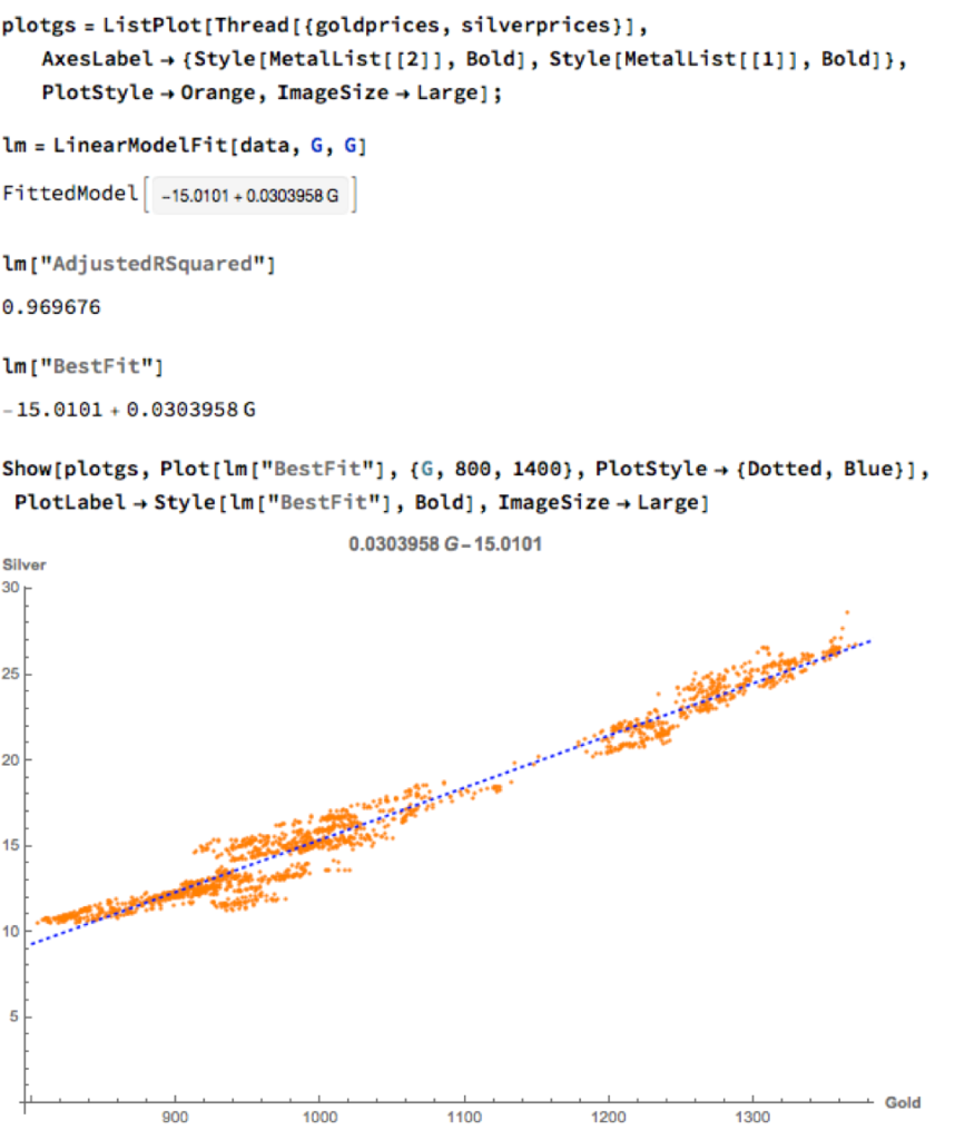
We can hope to do better with a standard linear model, regressing spot silver prices against spot gold prices. The fit of the best linear model is very good, with an R-sq of over 96%:
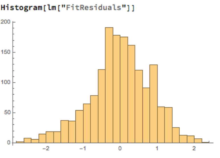
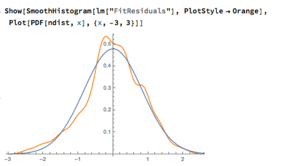
A trader might look to exploit the correlation relationship by selling silver when its market price is greater than the value estimated by the model (and buying when the model price exceeds the market price). Typically the spread is bought or sold when the log-price differential exceeds a threshold level that is set at twice the standard deviation of the price-difference series. The threshold levels derive from the assumption of Normality, which in fact does not apply here, as we can see from an examination of the residuals of the linear model:
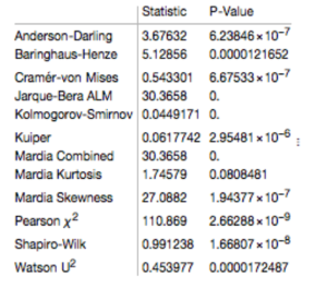
Given the evident lack of fit, especially in the left tail of the distribution, it is unsurprising that all of the formal statistical tests for Normality easily reject the null hypothesis:
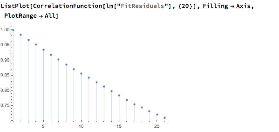
However, Normality, or the lack of it, is not the issue here: one could just as easily set the 2.5% and 97.5% percentiles of the empirical distribution as trade entry points. The real problem with the linear model is that it fails to take into account the time dependency in the price series. An examination of the residual autocorrelations reveals significant patterning, indicating that the model tends to under-or over-estimate the spot price of silver for long periods of time:
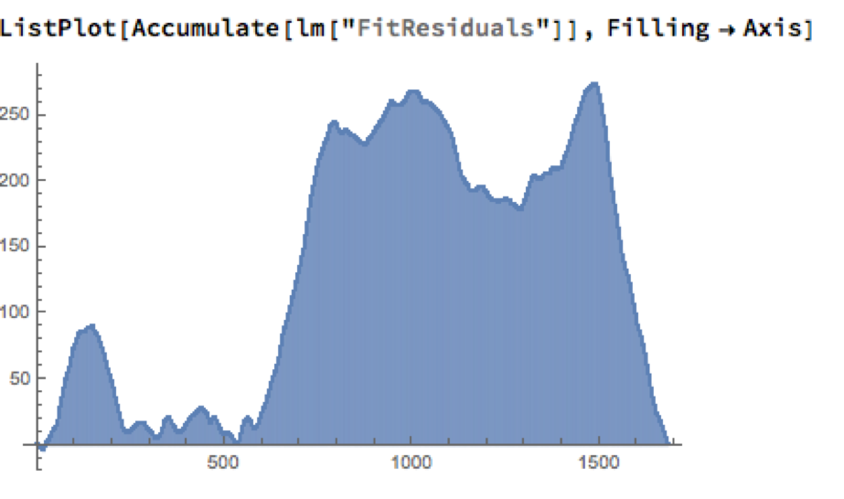
As the following chart shows, the cumulative difference between model and market prices can become very large indeed. A trader risks going bust waiting for the market to revert to model prices.
How does one remedy this? The shortcoming of the simple linear model is that, while it captures the interdependency between the price series very well, it fails to factor in the time dependency of the series. What is required is a model that will account for both features.
Multivariate Vector Autoregression Model
Rather than modeling the metal prices individually, or in pairs, we instead adopt a multivariate vector autoregression approach, modeling all three spot price processes together. The essence of the idea is that spot prices in each metal may be influenced, not only by historical values of the series, but also potentially by current and lagged prices of the other two metals.
Before proceeding we divide the data into two parts: an in-sample data set comprising data from 2012 to the end of 2015 and an out-of-sample period running from Jan-Aug 2016, which we use for model testing purposes. In what follows, I make the simplifying assumption that a vector autoregressive moving average process of order (1, 1) will suffice for modeling purposes, although in practice one would go through a procedure to test a wide spectrum of possible models incorporating moving average and autoregressive terms of varying dimensions.
In any event, our simplified VAR model is estimated as follows:
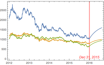
The chart below combines the actual, in-sample data from 2012-2015, together with the out-of-sample forecasts for each spot metal from January 2016.
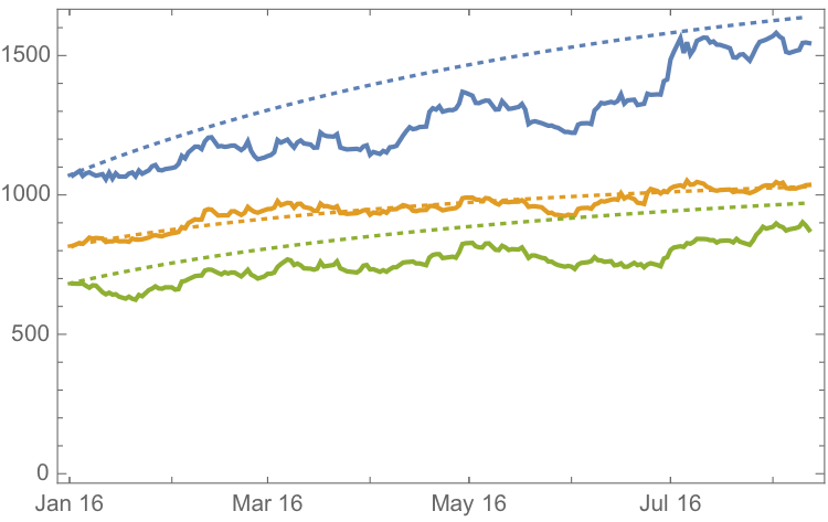
It is clear that the model projects a recovery in spot metal prices from the end of 2015. How did the forecasts turn out? In the chart below we compare the actual spot prices with the model forecasts, over the period from Jan to Aug 2016.
The actual and forecast percentage change in the spot metal prices over the out-of-sample period are as follows:
The VAR model does a good job of forecasting the strong upward trend in metal prices over the first eight months of 2016. It performs exceptionally well in its forecast of gold prices, although its forecasts for silver and platinum are somewhat over-optimistic. Nevertheless, investors would have made money taking a long position in any of the metals on the basis of the model projections.
Relative Value Trade
Another way to apply the model would be to implement a relative value trade, based on the model’s forecast that silver would outperform gold and platinum. Indeed, despite the model’s forecast of silver prices turning out to be over-optimistic, a relative value trade in silver vs. gold or platinum would have performed well: silver gained 44% in the period form Jan-Aug 2016, compared to only 26% for gold and 28% for platinum. A relative value trade entailing a purchase of silver and simultaneous sale of gold or platinum would have produced a gross return of 17% and 15% respectively.
A second relative value trade indicated by the model forecasts, buying platinum and selling gold, would have turned out less successfully, producing a gross return of less than 2%. We will examine the reasons for this in the next section.
Forecasts and Trading Opportunities Through 2016
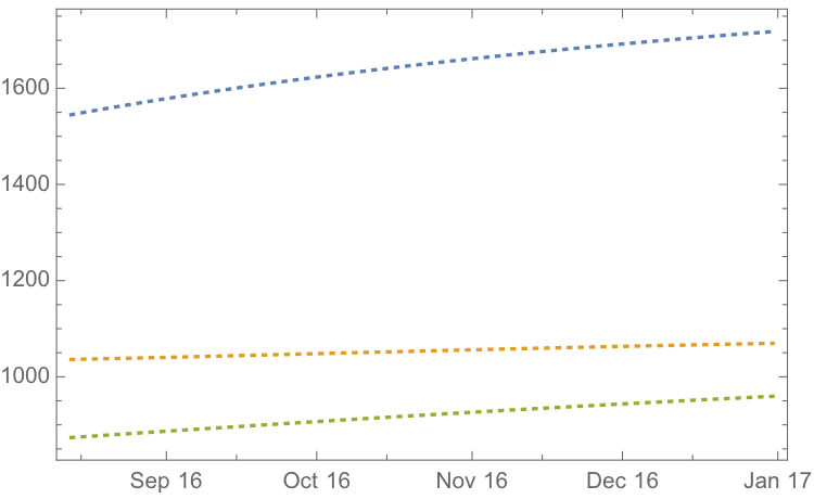
If we re-estimate the VAR model using all of the the available data through mid-Aug 2016 and project metal prices through the end of the year, the outcome is as follows:
While the positive trend in all three metals is forecast to continue, the new model (which incorporates the latest data) anticipates lower percentage rates of appreciation going forward:
Once again, the model predicts higher rates of appreciation for both silver and platinum relative to gold. So investors have the option to take a relative value trade, hedging a long position in silver or platinum with a short position in gold. While the forecasts for all three metals appear reasonable, the projections for platinum strike me as the least plausible.
The reason is that the major applications of platinum are industrial, most often as a catalyst: the metal is used as a catalytic converter in automobiles and in the chemical process of converting naphthas into higher-octane gasolines. Although gold is also used in some industrial applications, its demand is not so driven by industrial uses. Consequently, during periods of sustained economic stability and growth, the price of platinum tends to be as much as twice the price of gold, whereas during periods of economic uncertainty, the price of platinum tends to decrease due to reduced industrial demand, falling below the price of gold. Gold prices are more stable in slow economic times, as gold is considered a safe haven.
This is the most likely explanation of why the gold-platinum relative value trade has not worked out as expected hitherto and is perhaps unlikely to do so in the months ahead, as the slowdown in the global economy continues.
Conclusion
We have shown that simple models of the ratio or differential in the prices of precious metals are unlikely to provide a sound basis for forecasting or trading, due to non-stationarity and/or temporal dependencies in the residuals from such models.
On the other hand, a vector autoregression model that models all three price processes simultaneously, allowing both cross correlations and autocorrelations to be captured, performs extremely well in terms of forecast accuracy in out-of-sample tests over the period from Jan-Aug 2016.
Looking ahead over the remainder of the year, our updated VAR model predicts a continuation of the price appreciation, albeit at a slower rate, with silver and platinum expected to continue outpacing gold. There are reasons to doubt whether the appreciation of platinum relative to gold will materialize, however, due to falling industrial demand as the global economy cools.
Is Internal Bar Strength A Random Walk? The Case of Exxon-Mobil
For those who prefer a little more rigor in their quantitative research, I can offer more a somewhat more substantive statistical argument in favor of the IBS indicator discussed in my previous post.
Specifically, we can show quite convincingly that the IBS process is stationary, a highly desirable property much sought-after in, for example, the construction of statistical arbitrage strategies. Of course, by construction, the IBS is constrained to lie between the values of 0 and 1, so non-stationarity in the mean is highly unlikely. But, conceivably, there could be some time dependency in the process or in its variance, for instance. Then there is the further question as to whether the IBS indicator is mean-reverting, which would indicate that the underlying price process likewise has a tendency to mean revert.
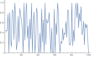
Let’s take the IBS series for Exxon-Mobil (XOM) as an example to work with. I have computed the series from the beginning of 1990, and the first 100 values are shown in the plot below.
Autocorrelation and Unit Root Tests
There appears to be little patterning in the process autocorrelations, and this is confirmed by formal statistical tests which fail to reject the null hypothesis that the first 20 autocorrelations are not, collectively, statistically significant.
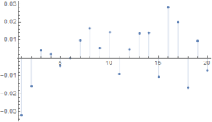
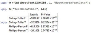
Next we test for the presence of a unit root in the IBS process (highly unlikely, given its construction) and indeed, unsurprisingly, the null hypothesis of a unit root is roundly rejected by the Dickey-Fuller and Phillips-Perron tests.
Variance Ratio Tests
We next conduct a formal test to determine whether the IBS series follows a random walk.
The variance ratio test assesses the null hypothesis that a univariate time series y is a random walk. The null model is
y(t) = c + y(t–1) + e(t),
where c is a drift constant (assumed zero for the IBS series) and e(t) are uncorrelated innovations with zero mean.
- When
IIDisfalse, the alternative is that the e(t) are correlated. - When
IIDistrue, the alternative is that the e(t) are either dependent or not identically distributed (for example, heteroscedastic).
We test whether the XOM IBS series is a random walk using various step sizes and perform the test with and without the assumption that the innovations are independent and identically distributed.
Switching to Matlab, we proceed as follows:
q = [2 4 8 2 4 8];
flag = logical([1 1 1 0 0 0]);
[h,pValue,stat,cValue,ratio] = vratiotest(XOMIBS,’period’,q,’IID’,flag)
Here h is a vector of Boolean decisions for the tests, with length equal to the number of tests. Values of h equal to 1 indicate rejection of the random-walk null in favor of the alternative. Values of h equal to 0 indicate a failure to reject the random-walk null.
The variable ratio is a vector of variance ratios, with length equal to the number of tests. Each ratio is the ratio of:
- The variance of the q-fold overlapping return horizon
- q times the variance of the return series
For a random walk, these ratios are asymptotically equal to one. For a mean-reverting series, the ratios are less than one. For a mean-averting series, the ratios are greater than one.
For the XOM IBS process we obtain the following results:
h = 1 1 1 1 1 1
pValue = 1.0e-51 * [0.0000 0.0000 0.0000 0.0000 0.0000 0.1027]
stat = -27.9267 -21.7401 -15.9374 -25.1412 -20.2611 -15.2808
cValue = 1.9600 1.9600 1.9600 1.9600 1.9600 1.9600
ratio = 0.4787 0.2405 0.1191 0.4787 0.2405 0.1191
The random walk hypothesis is convincingly rejected for both IID and non-IID error terms. The very low ratio values indicate that the IBS process is strongly mean reverting.
Conclusion
While standard statistical tests fail to find evidence of any non-stationarity in the Internal Bar Strength signal for Exxon-Mobil, the hypothesis that the series follows a random walk (with zero drift) is roundly rejected by variance ratio tests. These tests also confirm that the IBS series is strongly mean reverting, as we previously discovered empirically.
This represents an ideal scenario for trading purposes: a signal with the highly desirable properties that is both stationary and mean reverting. In the case of Exxon-Mobil, there appears to be clear evidence from both statistical tests and empirical trading strategies using the Internal Bar Strength indicator that the tendency of the price series to mean-revert is economically as well as statistically significant.


