Understanding Stock Price Range Forecasts

Stock Price Range Forecasts

Range forecasts are produced by estimating the parameters of a Geometric Brownian Motion process from historical data and using the model to project a large number of sample paths for the stock price over the coming month and year.

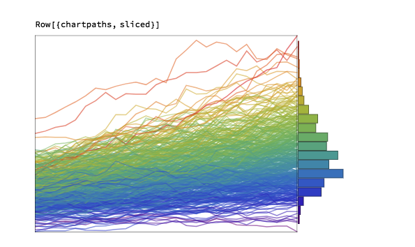
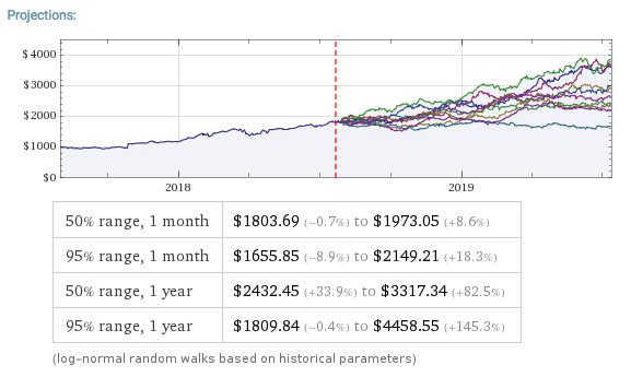
For example, this is a range forecast for Netflix, Inc. (NFLX) as at 7/27/2018 when the price of the stock stood at $355.21:

$NFLX

As you can see, the great majority of the simulated price paths trend upwards.  This is typical for most stocks on account of their upward drift, a tendency to move higher over time.  The statistical table below the chart tells you that in 50% of cases the ending stock price 1 month from the date of forecast was in the range $352.15 to $402.49. Similarly, around 50% of the time the price of the stock in one year’s time were found to be in the range $565.01 to $896.69.  Notice that the end points of the one-year range far exceed the end points of the one-month range forecast – again this is a feature of the upward drift in stocks.

If you want much greater certainty about the outcome, you should look at the 95% ranges.  So, for NFLX, the one month 95% range was projected to be $310.06 to $457.13.  Here, only 1 in 20 of the simulated price paths produced one month forecasts that were higher than $457.13, or lower than $310.06.

Notice that the spread of the one month and one year 95% ranges is much larger than of the corresponding 50% ranges.  This demonstrates the fundamental tradeoff between “accuracy” (the spread of the range) and “certainty”, (the probability of the outcome being with the projected range).  If you want greater certainty of the outcome, you have to allow for a broader span of possibilities, i.e. a wider range.

SSALGOTRADING AD

Uses of Range Forecasts

Most stock analysts tend to produce single price “targets”, rather than a range – these are known as “point forecasts” by econometricians.  So what’s the thinking behind range forecasts?

Range forecasts are arguably more useful than simple point forecasts.  Point forecasts make no guarantee as to the likelihood of the projected price – the only thing we know for sure about such forecasts is that they will be wrong!  Is the forecast target price optimistic or pessimistic?  We have no way to tell.

With range forecasts the situation is very different.  We can talk about the likelihood of a stock being within a specified range at a certain point in time.  If we want to provide a pessimistic forecast for the price in NFLX in one month’s time, for example, we could quote the value $352.15, the lower end of the 50% range forecast.  If we wanted to provide a very pessimistic forecast, one that is very likely to be exceeded, we could quote the bottom of the 95% range: $310.06.

The range also tells us about the future growth prospects for the firm.  So, for example, with NFLX, based on past performance, it is highly likely that the stock price will grow at a rate of more than 2.4% and, optimistically, might increase by almost 3x in the coming year (see the growth rates calculated for the 95% range values).

One specific use of range forecasts is in options trading.  If a trader is bullish on NFLX, instead of buying the stock, he might instead choose to sell one-month put options with a strike price below $352 (the lower end of the 50% one-month range).  If the trader wanted to be more conservative, he might look for put options struck at around $310, the bottom of the 95% range.  A more complex strategy might be to buy calls struck near the top of the 50% range, and sell more calls struck near the top of the 95% range (the theory being that the stock is quite likely to exceed the top of the 50% one-month range, but much less likely to reach the high end of the 95% range).

Limitations of Range Forecasts

Range forecasts are produced by using historical data to estimate the parameters of a particular type of mathematical model, known as a Geometric Brownian Motion process.  For those who are interested in the mechanics of how the forecasts are produced, I have summarized the relevant background theory below.

While there are grounds for challenging the use of such models in this context, it has to be acknowledged that the GBM process is one of the most successful mathematical models in finance today.  The problem lies not so much in the model, as in one of the key assumptions underpinning the approach:  specifically, that the characteristics of the stock process will remain as they are today (and as they have been in the historical past).  This assumption is manifestly untenable when applied to many stocks:  a company that was a high-growth $100M start-up is unlikely to demonstrate the same  rate of growth ten years later, as a $10Bn enterprise.  A company like Amazon that started out as an online book seller has fundamentally different characteristics today, as an online retail empire.  In such cases, forecasts about the future stock price – whether point or range forecasts – based on outdated historical informations are likely to be wrong, sometimes wildly so.

Having said that, there are a great many companies that have evolved to a point of relative stability over a period of perhaps several decades: for example, a company like Caterpillar Inc. (CAT).  In such cases the parameters of the GBM process underpinning the stock price are unlikely to fluctuate widely in the short term, so range forecasts are consequently more likely to be useful.

Another factor to consider are quarterly earnings reports, which can influence stock prices considerably in the short term, and corporate actions (mergers, takeovers, etc) that can change the long term characteristics of a firm and its stock price process in a fundamental way.  In these situations any forecast methodology is likely to unreliable, at least for a while, until the event has passed.  It’s best to avoid taking positions based on projections from historical data at times like this.

Review of Background Theory


GBM1

GBM2 GBM3 GBM4 GBM5

Riders on the Storm

The Worst Volatility Scare for Years

February 2018 was an insane month for stocks, wrote CNN:

A profound inflation scare. Not one but two 1,000-point plunges for the Dow. And a powerful comeback that almost went straight back up.

The CNN story-line continues:

The Dow plummeted more than 3,200 points, or 12%, in just two weeks. Then stocks raced back to life, at one point recovering about three-quarters of those losses.

Fittingly, February ended with more drama. The Dow tumbled 680 points during the month’s final two days, leaving it down about 1,600 points from the record high in late January.

The headline in the Financial Times was a little more nuanced, focusing on the impact of the market turmoil on quant hedge funds:


FT


Quant Funds Get Trashed

The FT reported:

Computer-driven, trend-following hedge funds are heading for their worst month in nearly 17 years after getting whipsawed when the stock market’s steady soar abruptly reversed into one of the quickest corrections in history earlier in February.

The carnage amongst hedge funds was widespread, according to the article:

Société Générale’s CTA index is down 5.55 per cent this month, even after the recent market rebound, making it the worst period for these systematic hedge funds since November 2001.
Man AHL’s $1.1bn Diversified fund lost almost 10 per cent in the month to February 16, while the London investment firm’s AHL Evolution and Alpha funds were down about 4-5 per cent over the same period. The flagship funds of GAM’s Cantab Capital, Systematica and Winton lost 9.5 per cent, 7.2 per cent and 4.6 per cent* respectively between the start of the month and February 16. Aspect Capital’s Diversified Fund dropped 9.5 per cent in the month to February 20, while a trend-following fund run by Lynx Asset Management slumped 12.7 per cent. A leveraged version of the same fund tumbled 18.8 per cent. One of the other big victims is Roy Niederhoffer, whose fund lost 21.1 per cent in the month to February 20.

Painful reading, indeed.


Traders conditioned to a state of somnambulance were shocked by the ferocity of the volatility spike, as the CBOE VIX index soared by over 200% in a single day, reaching a high of over 38 on Feb 5th:


VIX Index


Indeed, this turned out to be the largest ever two-day increase in the history of the index:

VIX_Spike_1

This Quant Strategy Made 27% In February Alone

So, for a quant-driven options strategy that is typically a premium seller, February must surely have been a disaster, if not a total wipe-out.  Not quite.  On the contrary, our Option Trader strategy made a massive gain of 27% for the month.  As a result strategy performance is now running at over 55% for 2018 YTD, while maintaining a Sharpe Ratio of 2.23.

Option Trader

You can tell that the strategy has a tendency to collect option premiums, not only because the strategy description says as much, but also from the observation that over 90% of strategy trades have been profitable – one of the defining characteristics of volatility strategies that are short-Vega, long-Theta.  The theory is that such strategies make money most of the time, but then give it all back (and more) when volatility inevitably spikes.  While that is generally true, in my experience, that clearly didn’t occur here.  So what’s the story?

One of the advantages of our Algo Trading Platform is that it not only reports in detail the live performance of our strategies, but it also reveals the actual trades on the site (typically delayed by 24-72 hours).  A review of the trades made by the Option Trader strategy from the end of January though early February indicates a strongly bullish bias, with short put trades in stocks such as Netflix, Inc. (NFLX), Shopify Inc. (SHOP), The Goldman Sachs Group, Inc. (GS) and Facebook, Inc. (FB), coupled with short call trades in VIX ETF products such as ProShares Ultra VIX Short-Term Futures (UVXY) and iPath S&P 500 VIX ST Futures ETN (VXX).  As volatility began to spike on 2/5, more calls were sold at increasingly fat premiums in several of the VIX Index ETFs.  These short volatility positions were later hedged with long trades in the underlying ETFs and, over time, both the hedges and the original option sales proved highly profitable. In other words, the extremely high levels of volatility enabled the strategy to profit on both legs of the trade, a highly unusual occurrence.  Meanwhile, while it was hedging its bets in the VIX ETF option trades, the strategy was becoming increasingly aggressive in the single stocks sector, taking outright long positions in Baidu, Inc. (BIDU), Align Technology, Inc. (ALGN), Netflix, Inc. (NFLX) and others, just as they became trading off their lows in the second week of the month.  By around Feb 12th the strategy recognized that the volatility shock had begun to subside and took advantage of the inflated option premia, selling puts across the board, in particular in the technology (Tesla, Inc. (TSLA), NVIDIA Corporation (NVDA)) and retail sectors (GrubHub Inc. (GRUB), Alibaba Group Holding Limited (BABA)) that had suffered especially heavy declines.  Many of these trades were closed at a substantial profit within a span of just a few days as the market stabilized and volatility subsided.  The strategy broadened the scope of its option selling as the month progressed, initially recovering the entirety of the drawdown it had initially suffered, before going on to register substantial profits on almost every trade.

To summarize:

  1.  Like many other market players, the Volatility Trader strategy was initially caught on the wrong side of the volatility spike and suffered a significant drawdown.
  2. Instead of liquidating positions, the strategy began hedging aggressively in sectors holding the greatest danger – VIX ETFs, in particular.  These trades ultimately proved profitable on both option and hedge legs as the market turned around and volatility collapsed.
  3. As soon as volatility showed signed of easing, the strategy began making aggressive bets on market stabilization and recovery, taking long positions in some of the most beaten-down stocks and selling puts across the board to capture inflated option premia.

Lesson Learned:  Aggressive Defense is the best Options Strategy in a Volatile Market

If there is one lesson above all others to be learned from this case study it is this:  that a period of market turmoil is a time of opportunity for option traders, but only if they play aggressively, both in defense and offense.  Many traders run scared at times like this and liquidate positions, taking heavy losses in the process that can prove impossible to recover from if, as here, the drawdown is severe.  This study shows that by holding one’s nerve and hedging rather than liquidating loss-making positions and then moving aggressively to capitalize on inflated option prices a trader can not only weather the storm but, as in this case, produce exceptional returns.

The key take-away is this: in order to play aggressively you have to have sufficient reserves in the tank to enable you to hold positions rather than liquidate them and, later on, to transition to selling expensive option premiums.  The mistake many option traders make is to trade too close to the line in term of margin limits, resulting  in a forced liquidation of positions that would otherwise have been profitable.

You can trade the Option Trader strategy live in your own brokerage account – go here for details.


Trading Prime Market Cycles

Magicicada tredecassini NC XIX male dorsal trim.jpg

Magicicada is the genus of the 13-year and 17-year periodical cicadas of eastern North America. Magicicada species spend most of their 13- and 17-year lives underground feeding on xylem fluids from the roots of deciduous forest trees in the eastern United States.  After 13 or 17 years, mature cicada nymphs emerge in the springtime at any given locality, synchronously and in tremendous numbers.  Within two months of the original emergence, the lifecycle is complete, the eggs have been laid, and the adult cicadas are gone for another 13 or 17 years.

The emergence period of large prime numbers (13 and 17 years) has been hypothesized to be a predator avoidance strategy adopted to eliminate the possibility of potential predators receiving periodic population boosts by synchronizing their own generations to divisors of the cicada emergence period. If, for example, the cycle length was, say, 12 years, then the species would be exposed to predators regenerating over cycles of 2, 3, 4, or 6 years.  Limiting their cycle to a large prime number reduces the variety of predators the species is likely to face.

SSALGOTRADING AD

Prime Cycles in Trading Strategies

What has any of this to do with trading?  When building a strategy in a particular market we might start by creating a model that works reasonably well on, say, 5-minute bars. Then, in order to improve the risk-adjusted returns we might try create a second sub-strategy on a different frequency.  This will hopefully result in a new series of signals, an increase in the number of trades, and corresponding improvement in the risk-adjusted returns of the overall strategy.  This phenomenon is referred to as temporal diversification.

What time frequency should we select for our second sub-strategy?  There are many factors to consider, of course, but one of them is that we would like to see as few duplicate signals between the two sub-strategies.  Otherwise we will simply be replicating trades, rather than reducing the overall level of strategy risk through temporal diversification.  The best way to minimize the overlap in signals generated by multiple sub-strategies is to use prime number bar frequencies (5 minute, 7 minute, 11 minute, etc).

S&P500 Swing Trading Strategy

An example of this approach is our EMini Swing Trading strategy which we operate on our Systematic Algotrading Platform.  This strategy is actually a combination of several different sub-strategies that operate on 5-minute, 11-minute, 17-minute and 31-minute bars.  Each strategy focuses on a different set of characteristics of the S&P 500 futures market, but the key point here is that the trading signals very rarely overlap and indeed several of the sub-strategies have a low correlation.

correl


The resulting increase in trade frequency and temporal diversification produces very attractive risk-adjusted performance: after an exceptional year in 2017 which saw a 78.58% net return, the strategy is already at  +60% YTD in 2018 and showing no sign of slowing down.

Investors can auto-trade the E-Mini Swing Trading strategy and many other strategies in their own account – see the Leaderboard for more details.

Perf1Monthly returns

Momentum Strategies

A few weeks ago I wrote an extensive post on a simple momentum strategy in E-Mini Futures. The basic idea is to buy the S&P500 E-Mini futures when the contract makes a new intraday high. This is subject to the qualification that the Internal Bar Strength fall below a selected threshold level. In order words, after a period of short-term weakness – indicated by the low reading of the Internal Bar Strength – we buy when the futures recover to make a new intraday high, suggesting continued forward momentum.

IBS is quite a useful trading indicator, which you can learn more about in the blog post:

A characteristic of momentum strategies is that they can often be applied successfully across several markets, usually with simple tweaks to the strategy parameters. As a case in point, take our Tech Momentum strategy, listed on the Systematic Strategies Algotrading platform which you can find out more about here:

This swing trading strategy applies similar momentum concepts to exploits long and short momentum effects in technology sector ETFs, focusing on the PROSHARES ULTRAPRO QQQ (TQQQ) and PROSHARES ULTRAPRO SHORT QQQ (SQQQ). Does it work? The results speak for themselves:

In four years of live trading the strategy has produced a compound annual return of 48.9%, with a Sharpe Ratio of 1.78 and Sortino Ratio of 2.98. 2018 is proving to be a banner year for the strategy, which is up by more than 48% YTD.

A very attractive feature of this momentum approach is that it is almost completely uncorrelated with the market and with a beta of just over 1 is hardly more risky than the market portfolio.

You can find out more about the Tech Momentum and other momentum strategies and how to trade them live in your own account on our Strategy Leaderboard:

New Algotrading Platform

Fig1


Systematic Strategies is pleased to announce the launch of its new Algo Trading Platform.  This will allow subscribers to follow a selection of our best strategies in equities, futures and options, for a low monthly subscription fee.

There is no minimum account size, and accounts of up to $250,000 can be traded on the platform.

The strategies are fully systematic and trades are executed automatically in your existing brokerage account, or you can open an account at one of our supported brokers, which include  Interactive Brokers, NinjaTrader, CQG, Gain Capital, AMP, Garwood, and many others.


Fig2


Find Strategies

Short LineFig3


Find Strategies


Short Line

FAQ1 FAQ2


More


Short Line

SYSTEMATIC STRATEGIES LLC

Systematic Strategies is an alternative investments firm utilizing quantitative modeling techniques to develop profitable trading strategies for deployment into global markets. Systematic Strategies seeks qualified investors as defined in Regulation D of the Securities Act of 1933. For information please contact us at info@ systematic-strategies.com or visit www.systematic-strategies.com.


RISK DISCLOSURE

This web site and the information contained herein is not and must not be construed as an offer to sell securities. Certain statements included in this web site, including, without limitation, statements regarding investment goals, strategies, and statements as to the manager’s expectations or opinions are forward-looking statements within the meaning of Section 27A of the Securities Act of 1933 (the “Securities Act”) and Section 21E of the Securities Exchange Act of 1944 (the “Exchange Act”) and are subject to risks and uncertainties. The factors discussed herein could cause actual results and development to be materially different from those expressed in or implied by such forward-looking statements. Accordingly, the information in this web site cannot be construed as to be guaranteed.

A Simple Momentum Strategy

Momentum trading strategies span a diverse range of trading ideas.  Often they will use indicators to determine the recent underlying trend and try to gauge the strength of the trend using measures of the rate of change in the price of the asset.

One very simple momentum concept, a strategy in S&P500 E-Mini futures, is described in the following blog post:

http://www.quantifiedstrategies.com/buy-when-sp-500-makes-new-intraday-high/

The basic idea is to buy the S&P500 E-Mini futures when the contract makes a new intraday high.  This is subject to the qualification that the Internal Bar Strength fall below a selected threshold level.  In order words, after a period of short-term weakness – indicated by the low reading of the Internal Bar Strength – we buy when the futures recover to make a new intraday high, suggesting continued forward momentum.

IBS is quite a useful trading indicator, which you can learn more about in these posts:

http://jonathankinlay.com/2016/06/the-internal-bar-strength-indicator/

http://jonathankinlay.com/2016/06/quick-note-internal-bar-strength-stationarity/


I have developed a version of the intraday-high strategy, using parameters to generalize it and allow for strategy optimization.  The Easylanguage code for my version of the strategy is as follows:

Inputs:
nContracts(1),
ndaysHigh(5),
IBSlag(1),
IBStrigger(0.15);

Vars:

IBS(0.5);

If H[IBSlag] > L[IBSlag] then
Begin
IBS=(H[IBSlag]-C[IBSlag])/(H[IBSlag]-L[IBSlag]);
end;
If (IBS <= IBStrigger) and (H[0] >= Highest(High, ndaysHigh)) then
begin
Buy nContracts contracts this bar on close;
end;

If C[0] > H[1] then
begin
Sell all contracts this bar on close;
end;

The performance results for the strategy appear quite promising, despite the downturn in strategy profitability in 2018 to date (all performance results are net of slippage and commission):


Fig1 Fig3

Fig2


SSALGOTRADING AD

Robustness Testing with Walk Forward Optimization

We evaluate the robustness of the strategy using the  Walk Forward Optimization feature in Tradestation.  Walk forward analysis is the process of optimizing a trading system using a limited set of parameters, and then testing the best optimized parameter set on out-of-sample data. This process is similar to how a trader would use an automated trading system in real live trading. The in-sample time window is shifted forward by the period covered by the out-of-sample test, and the process is repeated. At the end of the test, all of the recorded results are used to assess the trading strategy.

In other words, walk forward analysis does optimization on a training set; tests on a period after the set and then rolls it all forward and repeats the process. This gives a larger out-of-sample period and allows the system developer to see how stable the system is over time.

The  image below illustrates the walk forward analysis procedure. An optimization is performed over a longer period (the in-sample data), and then the optimized parameter set is tested over a subsequent shorter period (the out-of-sample data). The optimization and testing periods are shifted forward, and the process is repeated until a suitable sample size is achieved.


WFO


Tradestation enables the user to run a battery of WFO tests, using different size in-sample and out-of-sample sizes and number of runs.  The outcome of each test is evaluated on several specific criteria such as the net profit and drawdown and only if the system meets all of the criteria is the test designated as a “Pass”.  This gives the analyst a clear sense of the robustness of his strategy across multiple periods and sample sizes.

A WFO cluster analysis summary for the momentum strategy is illustrated below.  The cluster test is designated as “Failed” overall, since the strategy failed to meet the test criteria for a preponderance of the individual walk-forward tests.  The optimal parameters found in each test vary considerably over the sample periods spanning 2003-2018, giving concerns about the robustness of the strategy under changing market conditions.

Fig4


Improving the Strategy

We can improve both the performance and robustness of our simple momentum strategy by combining it with several other trend and momentum indicators. One such example is illustrated in the performance charts and tables below.  The strategy has performed well in both bull and bear markets and in both normal and volatile market conditions:


Fig5 Fig6

Fig7

A WFO cluster analysis indicates that the revised momentum strategy is highly robust to the choice of sample size and strategy parameters, as it passes every test in the 30-cell WFO analysis cluster table:

Fig8


Conclusion

Momentum strategies are well known and easy to develop using standard methodologies, such as the simple indicators used in this example. They tend to work well in most equity index futures markets, and in some commodity markets too.  One of their big drawbacks, however, is that they typically go through periods of poor performance and need to be tested thoroughly for robustness in order to ensure satisfactory results under the full range of market conditions.

Finding Alpha in 2018

Given the current macro-economic environment, where should investors focus their search for sources of alpha in the year ahead?  By asking enough economists or investment managers you will find as many different opinions on the subject as would care to, no doubt many of them conflicting.  These are some thoughts on the subject from my perspective, as a quantitative hedge fund manager.

SSALGOTRADING AD

Global Market Performance in 2017

Let’s begin by reviewing some of the best and worst performing assets of 2017 (I am going to exclude cryptocurrencies from the ensuing discussion).  Broadly speaking, the story across the piste has been one of strong appreciation in emerging markets, both in equities and currencies, especially in several of the Eastern European economies.  In Government bond markets Greece has been the star of the show, having stepped back from the brink of the economic abyss.  Overall, international diversification has been a key to investment success in 2017 and I believe that pattern will hold in 2018.

BestWorstEquityMkts2017

BestWorstCurrencies2017

BestWorstGvtBond


US Yield Curve and Its Implications

Another key development that investors need to take account of is the extraordinary degree of flattening of the yield curve in US fixed income over the course of 2017:

YieldCurve


This process has now likely reached the end point and will begin to reverse as the Fed and other central banks in developed economies start raising rates.  In 2018 investors should seek to protect their fixed income portfolios by shortening duration, moving towards the front end of the curve.

US Volatility and Equity Markets

A prominent feature of US markets during 2017 has been the continuing collapse of equity index volatility, specifically the VIX Index, which reached an all-time low of 9.14 in November and continues to languish at less than half the average level of the last decade:

VIX Index

Source: Wolfram Alpha

One consequence of the long term decline in volatility has been to drastically reduce the profitability of derivatives markets, for both traders and market makers. Firms have struggled to keep up with the high cost of technology and the expense of being connected to the fragmented U.S. options market, which is spread across 15 exchanges. Earlier in 2017, Interactive Brokers Group Inc. sold its Timber Hill options market-making unit — a pioneer of electronic trading — to Two Sigma Securities.   Then, in November, Goldman Sachs announced it was shuttering its option market making business in US exchanges, citing high costs, sluggish volume and low volatility.

The impact has likewise been felt by volatility strategies, which performed well in 2015 and 2016, only to see returns decline substantially in 2017.  Our own Systematic Volatility strategy, for example, finished the year up only 8.08%, having produced over 28% in the prior year.

One side-effect of low levels of index volatility has been a fall in stock return correlations, and, conversely, a rise in the dispersion of stock returns.   It turns out that index volatility and stock correlation are themselves correlated and indeed, cointegrated:

http://jonathankinlay.com/2017/08/correlation-cointegration/


In simple terms, stocks have a tendency to disperse more widely around an increasingly sluggish index.  The “kinetic energy” of markets has to disperse somewhere and if movements in the index are muted then relative movement in individual equity returns will become more accentuated.  This is an environment that ought to favor stock picking and both equity long/short and market neutral strategies  should outperform.  This certainly proved to be the case for our Quantitative Equity long/short strategy, which produced a net return of 17.79% in 2017, but with an annual volatility of under 5%:

QE Perf


Looking ahead to 2018, I expect index volatility and equity correlations rise as  the yield curve begins to steepen, producing better opportunities for volatility strategies.  Returns from equity long/short and market neutral strategies may moderate a little as dispersion diminishes.

Futures Markets

Big increases in commodity prices and dispersion levels also lead to improvements in the performance of many CTA strategies in 2017. In the low frequency space our Futures WealthBuilder strategy produced a net return of 13.02% in 2017, with a Sharpe Ratio above 3 (CAGR from inception in 2013 is now at 20.53%, with an average annual standard deviation of 6.36%).  The star performer, however, was our High Frequency Futures strategy.  Since launch in March 2017 this has produce a net return of 32.72%, with an annual standard deviation of 5.02%, on track to generate an annual Sharpe Ratio above 8 :

HFT Perf

Looking ahead, the World Bank has forecast an increase of around 4% in energy prices during 2018, with smaller increases in the price of agricultural products.   This is likely to be helpful to many CTA strategies, which will likely see further enhancements in performance over the course of the year.  Higher frequency strategies are more dependent on commodity market volatility, which is seen more likely to rise than fall in the year ahead.

Conclusion

US fixed income investors are likely to want to shorten duration as the yield curve begins to steepen in 2018, bringing with it higher levels of index volatility that will favor equity high frequency and volatility strategies.  As in 2017, there is likely much benefit to be gained in diversifying across international equity and currency markets.  Strengthening energy prices are likely to sustain higher rates of return in futures strategies during the coming year.

Trading Bitcoin

At Systematic Strategies we have developed a brilliant, new investment strategy.  We call it buying Bitcoin.  It works like this:  you take some of your hard-earned fiat and use it to buy Bitcoin.  Then, a week or two later, you do the same thing all over again.   So far the strategy is up around 400% YTD.  Genius.

It’s such a successful strategy that we are tempted to clone it.  Buying Litecoin, or Ethereum, spring to mind.

As freshly-minted, bona-fide cryptocurrency entrepreneurs, it is perhaps timely to ponder the roots of this success story and share our discoveries with other, perhaps more rational investors, who may be inclined to treat the whole cryptocurrency malarky as a tulip-Ponzi scheme.  First, there is a back-story to this.  During tulipmaniathe mid 1990’s I was teaching computational finance at Carnegie Mellon to some very bright students who were, naturally enough, playing the market on the side.  This was the time of the internet boom with tech stocks like Amazon, Ebay, Sun Microsystems, et al, leading the charge to ever higher levels in the market.  The multiples that some of these stocks were trading at were truly astonishing.  I had seen something similar just before the crash in the Japanese market towards the end of the 1980’s, when stocks were trading at three-figure multiples.  So by around 1997/98 I was becoming increasingly nervous that the tech boom might be at the point of imminent collapse.  I conveyed these sentiments to my students, expressing concern that they should not over-commit themselves to what might turn out to be a bubble.  My advice was roundly ignored and for the next couple of years I suffered the almost daily humiliation of watching the market indices reach even higher levels, to the joy of dot com investors.  When the crash came many lost most, if not all, of their investment.  It was like a funeral in the Hamptons that summer. Teary-eyed students asked me for advice as to what they should do to salvage what was left of their investment nest egg.  I didn’t have the stomach for gloating.  The only piece of advice I could think to offer them was:  “learn”.  I hope they did.  Because here we are again.

SSALGOTRADING AD

What concerned me back in ’98 was not that I didn’t understand the importance of the new internet paradigm:  on the contrary, I was an early adopter of the new technologies.  I fully understood the potential benefits that a digital business like Amazon enjoyed versus bricks and mortar rivals.  But it’s also the case that I under-estimated the potential of a company like Amazon, in several important ways.  For instance, I did not foresee how useful and important customer reviews would become (facilitated by the digital medium); nor did I anticipate Amazon being as successful as it has been in broadening the scope of its services from books (then) to just about everything (now); and I also under-estimated the challenge that the new entrants would pose to traditional rivals, who struggled (and often failed) to adapt their hitherto successful business strategies.  In other words, my concern didn’t stem from a lack of appreciation of the potential of the new tech  companies, although I certainly under-estimated that potential in some cases.  Rather, my thinking was that it had gone too far, too fast and that the blistering pace of the market melt-up would inevitably slow.  I was right, but way too early.  It is notoriously difficult to get the timing of the bubble-popping right, even if the call is correct.

Bitcoin Chart


Chaotic trading marks new surge in bitcoin price

In one wild 20 minute period, the price of bitcoin soared $2,000 per coin to more than $19,000 only to drop to $15,000 on the Coinbase trading venue.  – Financial Times, Dec 8th, 2017


So to Bitcoin, which is undergoing a similar melt-up.  Again, the rationale for the popularity of cryptocurrencies is not hard to fathom, given all the central bank shenanigans of the last decade and the poor reputation that several major banks have earned as serial manipulators of markets in fiat currency substitutes, like gold, or silver.  Once again, it appears to me, the entities whose well established business models are most threatened by the arrival of cryptocurrencies have been slow on the uptake and most, like JP Morgan, for instance, are still in denial.  The chief threat from cryptocurrencies lies in their potential to dis-intermediate the banks, by allowing users to transact directly with one another, and also Governments, who stand to lose considerable sums in tax revenue.  No doubt they will eventually wake up to the scale of threat that Bitcoin poses and respond accordingly in due course – i.e. expect an avalanche of new regulation and government propaganda seeking to equate ownership of Bitcoin with “money laundering”, whatever that preposterous phrase might actually mean. I am not convinced that the genie can be stuffed back into the bottle so easily.

Given the value and scale of the market that cryptocurrencies are in the process of disrupting, i.e. global banking and taxation, the upside potential is indeed enormous. I fully expect the surge to continue for some time.  But we can expect a great deal of volatility and several corrections of 20%, or more, along the way.  The first of these might arrive next week, as Bitcoin futures start trading, enabling speculators to initiate short positions against the cryptocurrency.  Other adverse events are likely to include increased scrutiny by government agencies like the IRS and market regulators like the SEC, although it remains to be seen how effectively they are able to operate in this sphere.

Bitcoin-trading

So, with all that said, here are some thoughts on how to play the market, if you must:

  1.  Check out this useful Beginner’s Guide to Trading Bitcoin
  2. Invest no more than 10% to 20% of your net worth.  Losing this will hurt, but not kill you.  Yes, you probably won’t become a Bitcoin billionaire, but neither will you end up in the poor house.  Do not, under any circumstances, sell all your assets and plunge in.  If you lose your home and the college fund, your wife and kids will never forgive you.
  3. Wait to see if we get a decent pullback after futures trading starts before you buy (more).  If that doesn’t happen, it’s up to you to decide whether  you want to wait it out or get aboard the train immediately.  There is no right answer.  At some point you are going to lose at least 20% of the value of your investment.  It could be on day one, or six months from now.  There is no way to know.
  4. I have read a few articles by traders threatening to short the heck out of the futures market as soon as it opens.  For some of them this appears to be revenge for having missed a golden opportunity to buy Bitcoin when it was worth a fraction of the price it trades at today.  Please don’t do this.  It will be like trying to stop a freight train with your hand.   You might get lucky, once or twice, but sooner or later you are going to get run over.  And it will hurt a lot.
  5. If you want to trade the short side, or trade the long side more conservatively, consider a pairs trade.  By this I mean, for instance, if you do decide to sell Bitcoin futures, consider hedging the position by buying another cryptocurrency like Ethereum or Litecoin.  For a detailed description of how to approach this in a more sophisticated way, see these posts:

http://jonathankinlay.com/2017/03/pairs-trading-copulas/


http://jonathankinlay.com/2015/02/developing-statistical-arbitrage-strategies-using-cointegration/

DISCLAIMER

As always, readers are entirely responsible for making their own investment decisions and for any and all consequences arising from them.  The author bears no responsibility for any action or decision taken, or not taken, by any investor pursuant to this or other articles and disclaims any responsibility for investment decisions taken by readers of this blog.