Finding Alpha in 2018

Given the current macro-economic environment, where should investors focus their search for sources of alpha in the year ahead?  By asking enough economists or investment managers you will find as many different opinions on the subject as would care to, no doubt many of them conflicting.  These are some thoughts on the subject from my perspective, as a quantitative hedge fund manager.

SSALGOTRADING AD

Global Market Performance in 2017

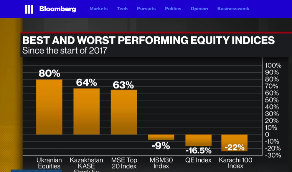
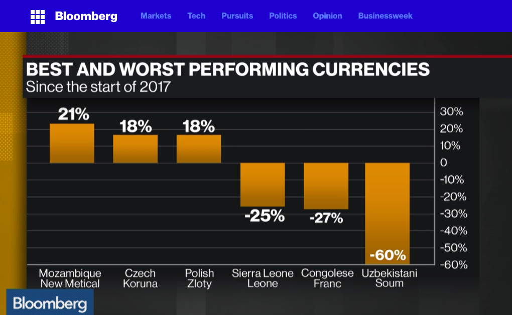
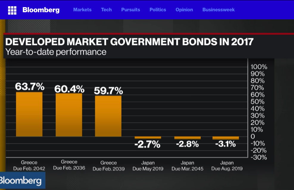
Let’s begin by reviewing some of the best and worst performing assets of 2017 (I am going to exclude cryptocurrencies from the ensuing discussion).  Broadly speaking, the story across the piste has been one of strong appreciation in emerging markets, both in equities and currencies, especially in several of the Eastern European economies.  In Government bond markets Greece has been the star of the show, having stepped back from the brink of the economic abyss.  Overall, international diversification has been a key to investment success in 2017 and I believe that pattern will hold in 2018.

BestWorstEquityMkts2017

BestWorstCurrencies2017

BestWorstGvtBond


US Yield Curve and Its Implications

Another key development that investors need to take account of is the extraordinary degree of flattening of the yield curve in US fixed income over the course of 2017:

YieldCurve


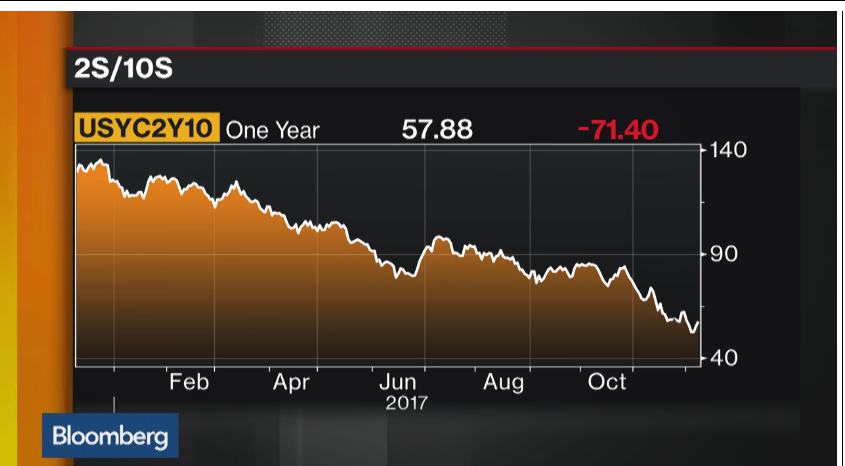
This process has now likely reached the end point and will begin to reverse as the Fed and other central banks in developed economies start raising rates.  In 2018 investors should seek to protect their fixed income portfolios by shortening duration, moving towards the front end of the curve.

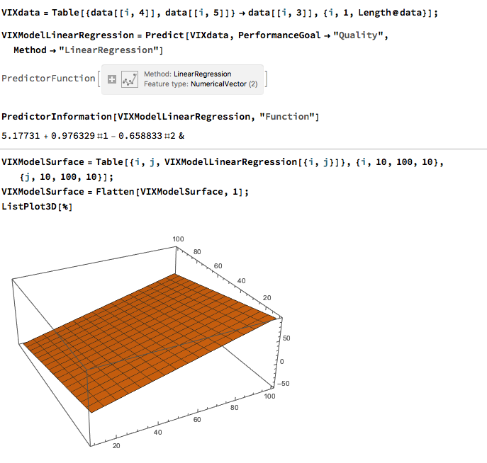
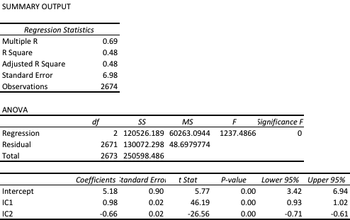
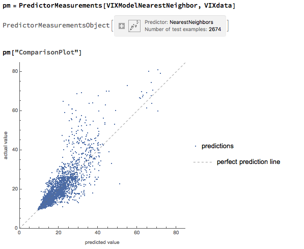
US Volatility and Equity Markets

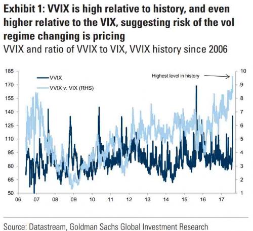
A prominent feature of US markets during 2017 has been the continuing collapse of equity index volatility, specifically the VIX Index, which reached an all-time low of 9.14 in November and continues to languish at less than half the average level of the last decade:

VIX Index

Source: Wolfram Alpha

One consequence of the long term decline in volatility has been to drastically reduce the profitability of derivatives markets, for both traders and market makers. Firms have struggled to keep up with the high cost of technology and the expense of being connected to the fragmented U.S. options market, which is spread across 15 exchanges. Earlier in 2017, Interactive Brokers Group Inc. sold its Timber Hill options market-making unit — a pioneer of electronic trading — to Two Sigma Securities.   Then, in November, Goldman Sachs announced it was shuttering its option market making business in US exchanges, citing high costs, sluggish volume and low volatility.

The impact has likewise been felt by volatility strategies, which performed well in 2015 and 2016, only to see returns decline substantially in 2017.  Our own Systematic Volatility strategy, for example, finished the year up only 8.08%, having produced over 28% in the prior year.

One side-effect of low levels of index volatility has been a fall in stock return correlations, and, conversely, a rise in the dispersion of stock returns.   It turns out that index volatility and stock correlation are themselves correlated and indeed, cointegrated:

http://jonathankinlay.com/2017/08/correlation-cointegration/


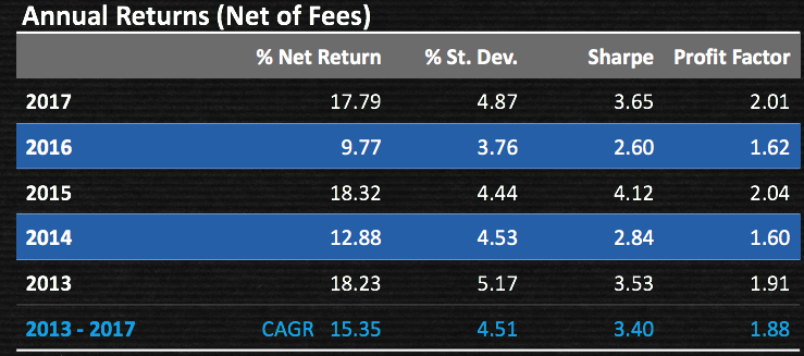
In simple terms, stocks have a tendency to disperse more widely around an increasingly sluggish index.  The “kinetic energy” of markets has to disperse somewhere and if movements in the index are muted then relative movement in individual equity returns will become more accentuated.  This is an environment that ought to favor stock picking and both equity long/short and market neutral strategies  should outperform.  This certainly proved to be the case for our Quantitative Equity long/short strategy, which produced a net return of 17.79% in 2017, but with an annual volatility of under 5%:

QE Perf


Looking ahead to 2018, I expect index volatility and equity correlations rise as  the yield curve begins to steepen, producing better opportunities for volatility strategies.  Returns from equity long/short and market neutral strategies may moderate a little as dispersion diminishes.

Futures Markets

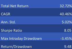
Big increases in commodity prices and dispersion levels also lead to improvements in the performance of many CTA strategies in 2017. In the low frequency space our Futures WealthBuilder strategy produced a net return of 13.02% in 2017, with a Sharpe Ratio above 3 (CAGR from inception in 2013 is now at 20.53%, with an average annual standard deviation of 6.36%).  The star performer, however, was our High Frequency Futures strategy.  Since launch in March 2017 this has produce a net return of 32.72%, with an annual standard deviation of 5.02%, on track to generate an annual Sharpe Ratio above 8 :

HFT Perf

Looking ahead, the World Bank has forecast an increase of around 4% in energy prices during 2018, with smaller increases in the price of agricultural products.   This is likely to be helpful to many CTA strategies, which will likely see further enhancements in performance over the course of the year.  Higher frequency strategies are more dependent on commodity market volatility, which is seen more likely to rise than fall in the year ahead.

Conclusion

US fixed income investors are likely to want to shorten duration as the yield curve begins to steepen in 2018, bringing with it higher levels of index volatility that will favor equity high frequency and volatility strategies.  As in 2017, there is likely much benefit to be gained in diversifying across international equity and currency markets.  Strengthening energy prices are likely to sustain higher rates of return in futures strategies during the coming year.

Modeling Volatility and Correlation

In a previous blog post I mentioned the VVIX/VIX Ratio, which is measured as the ratio of the CBOE VVIX Index to the VIX Index. The former measures the volatility of the VIX, or the volatility of volatility.

http://jonathankinlay.com/2017/07/market-stress-test-signals-danger-ahead/

A follow-up article in ZeroHedge shortly afterwards pointed out that the VVIX/VIX ratio had reached record highs, prompting Goldman Sachs analyst Ian Wright to comment that this could signal the ending of the current low-volatility regime:

vvix to vix 2_0


A linkedIn reader pointed out that individual stock volatility was currently quite high and when selling index volatility one is effectively selling stock correlations, which had now reached historically low levels. I concurred:

What’s driving the low vol regime is the exceptionally low level of cross-sectional correlations. And, as correlations tighten, index vol will rise. Worse, we are likely to see a feedback loop – higher vol leading to higher correlations, further accelerating the rise in index vol. So there is a second order, Gamma effect going on. We see that is the very high levels of the VVIX index, which shot up to 130 last week. The all-time high in the VVIX prior to Aug 2015 was around 120. The intra-day high in Aug 2015 reached 225. I’m guessing it will get back up there at some point, possibly this year.

SSALGOTRADING AD

As there appears to be some interest in the subject I decided to add a further blog post looking a little further into the relationship between volatility and correlation.  To gain some additional insight we are going to make use of the CBOE implied correlation indices.  The CBOE web site explains:

Using SPX options prices, together with the prices of options on the 50 largest stocks in the S&P 500 Index, the CBOE S&P 500 Implied Correlation Indexes offers insight into the relative cost of SPX options compared to the price of options on individual stocks that comprise the S&P 500.

  • CBOE calculates and disseminates two indexes tied to two different maturities, usually one year and two years out. The index values are published every 15 seconds throughout the trading day.
  • Both are measures of the expected average correlation of price returns of S&P 500 Index components, implied through SPX option prices and prices of single-stock options on the 50 largest components of the SPX.

Dispersion Trading

One application is dispersion trading, which the CBOE site does a good job of summarizing:

The CBOE S&P 500 Implied Correlation Indexes may be used to provide trading signals for a strategy known as volatility dispersion (or correlation) trading. For example, a long volatility dispersion trade is characterized by selling at-the-money index option straddles and purchasing at-the-money straddles in options on index components. One interpretation of this strategy is that when implied correlation is high, index option premiums are rich relative to single-stock options. Therefore, it may be profitable to sell the rich index options and buy the relatively inexpensive equity options.

The VIX Index and the Implied Correlation Indices

Again, the CBOE web site is worth quoting:

The CBOE S&P 500 Implied Correlation Indexes measure changes in the relative premium between index options and single-stock options. A single stock’s volatility level is driven by factors that are different from what drives the volatility of an Index (which is a basket of stocks). The implied volatility of a single-stock option simply reflects the market’s expectation of the future volatility of that stock’s price returns. Similarly, the implied volatility of an index option reflects the market’s expectation of the future volatility of that index’s price returns. However, index volatility is driven by a combination of two factors: the individual volatilities of index components and the correlation of index component price returns.

Let’s dig into this analytically.  We first download and plot the daily for the VIX and Correlation Indices from the CBOE web site, from which it is evident that all three series are highly correlated:

Fig1

An inspection reveals significant correlations between the VIX index and the two implied correlation indices, which are themselves highly correlated.  The S&P 500 Index is, of course, negatively correlated with all three indices:

Fig8

Modeling Volatility-Correlation

The response surface that describes the relationship between the VIX index and the two implied correlation indices is locally very irregular, but the slope of the surface is generally positive, as we would expect, since the level of VIX correlates positively with that of the two correlation indices.

Fig2

The most straightforward approach is to use a simple linear regression specification to model the VIX level as a function of the two correlation indices.  We create a VIX Model Surface object using this specification with the  Mathematica Predict function:Fig3The linear model does quite a good job of capturing the positive gradient of the response surface, and in fact has a considerable amount of explanatory power, accounting for a little under half the variance in the level of the VIX index:

Fig 4

However, there are limitations.  To begin with, the assumption of independence between the explanatory variables, the correlation indices, clearly does not hold.  In cases such as this, where explanatory variables are multicolinear, we are unable to draw inferences about the explanatory power of individual regressors, even though the model as a whole may be highly statistically significant, as here.

Secondly, a linear regression model is not going to capture non-linearities in the volatility-correlation relationship that are evident in the surface plot.  This is confirmed by a comparison plot, which shows that the regression model underestimates the VIX level for both low and high values of the index:

Fig5

We can achieve a better outcome using a machine learning algorithm such as nearest neighbor, which is able to account for non-linearities in the response surface:

Fig6

The comparison plot shows a much closer correspondence between actual and predicted values of the VIX index,  even though there is evidence of some remaining heteroscedasticity in the model residuals:

Fig7

Conclusion

A useful way to think about index volatility is as a two dimensional process, with time-series volatility measured on one dimension and dispersion (cross-sectional volatility, the inverse of correlation) measured on the second.  The two factors are correlated and, as we have shown here, interact in a complicated, non-linear way.

The low levels of index volatility we have seen in recent months result, not from low levels of volatility in component stocks, but in the historically low levels of correlation (high levels of dispersion) in the underlying stock returns processes. As correlations begin to revert to historical averages, the impact will be felt in an upsurge in index volatility, compounded by the non-linear interaction between the two factors.