Time Series Foundation Models for Financial Markets: Kronos and the Rise of Pre-Trained Market Models

The quant finance industry has spent decades building specialized models for every conceivable forecasting task: GARCH variants for volatility, ARIMA for mean reversion, Kalman filters for state estimation, and countless proprietary approaches for statistical arbitrage. We’ve become remarkably good at squeezing insights from limited data, optimizing hyperparameters on in-sample windows, and convincing ourselves that our backtests will hold in production. Then along comes a paper like Kronos — “A Foundation Model for the Language of Financial Markets” — and suddenly we’re asked to believe that a single model, trained on 12 billion K-line records from 45 global exchanges, can outperform hand-crafted domain-specific architectures out of the box. That’s a bold claim. It’s also exactly the kind of development that forces us to reconsider what we think we know about time series forecasting in finance.

The Foundation Model Paradigm Comes to Finance

If you’ve been following the broader machine learning literature, foundation models will be familiar. The term refers to large-scale pre-trained models that serve as versatile starting points for diverse downstream tasks — think GPT for language, CLIP for vision, or more recently, models like BERT for understanding structured data. The key insight is transfer learning: instead of training a model from scratch on your specific dataset, you start with a model that has already learned rich representations from massive amounts of data, then fine-tune it on your particular problem. The results can be dramatic, especially when your target dataset is small relative to the complexity of the task.

Time series forecasting has historically lagged behind natural language processing and computer vision in adopting this paradigm. Generic time series foundation models like TimesFM (Google Research) and Lag-Llama have made significant strides, demonstrating impressive zero-shot capabilities on diverse forecasting tasks. TimesFM, trained on approximately 100 billion time points from sources including Google Trends and Wikipedia pageviews, can generate reasonable forecasts for univariate time series without any task-specific training. Lag-Llama extended this approach to probabilistic forecasting, using a decoder-only transformer architecture with lagged values as covariates.

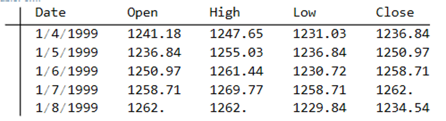
But here’s the problem that the Kronos team identified: generic time series foundation models, despite their scale, often underperform dedicated domain-specific architectures when evaluated on financial data. This shouldn’t be surprising. Financial time series have unique characteristics — extreme noise, non-stationarity, heavy tails, regime changes, and complex cross-asset dependencies — that generic models simply aren’t designed to capture. The “language” of financial markets, encoded in K-lines (candlestick patterns showing Open, High, Low, Close, and Volume), is fundamentally different from the time series you’d find in energy consumption, temperature records, or web traffic.

Enter Kronos: A Foundation Model Built for Finance

Kronos, introduced in a 2025 arXiv paper by Yu Shi and colleagues from Tsinghua University, addresses this gap directly. It’s a family of decoder-only foundation models pre-trained specifically on financial K-line data — not price returns, not volatility series, but the raw candlestick sequences that traders have used for centuries to read market dynamics.

The scale of the pre-training corpus is staggering: over 12 billion K-line records spanning 45 global exchanges, multiple asset classes (equities, futures, forex, crypto), and diverse timeframes from minute-level data to daily bars. This is not a model that has seen a few thousand time series. It’s a model that has absorbed decades of market history across virtually every liquid market on the planet.

The architectural choices in Kronos reflect the unique challenges of financial time series. Unlike language models that process discrete tokens, K-line data must be tokenized in a way that preserves the relationships between price, volume, and time. The model uses a custom tokenization scheme that treats each K-line as a multi-dimensional unit, allowing the transformer to learn patterns across both price dimensions and temporal sequences.

What Makes Kronos Different: Architecture and Methodology

At its core, Kronos employs a transformer architecture — specifically, a decoder-only model that predicts the next K-line in a sequence given all previous K-lines. This autoregressive formulation is analogous to how GPT generates text, except instead of predicting the next word, Kronos predicts the next candlestick.

The mathematical formulation is worth understanding in detail. Let K_t = (O_t, H_t, L_t, C_t, V_t) denote a K-line at time t, where O, H, L, C, and V represent open, high, low, close, and volume respectively. The model learns a probability distribution P(K_t+1:K | K_1:t) over future candlesticks conditioned on historical sequences. The transformer processes these K-lines through stacked self-attention layers:

$h^{(l)} = \text{Attention}(Q^{(l)}, K^{(l)}, V^{(l)}) + h^{(l-1)}$

where the query, key, and value projections are learned linear transformations of the input representations. The attention mechanism computes:

$\text{Attention}(Q, K, V) = \text{softmax}\left(\frac{QK^T}{\sqrt{d_k}}\right)V$

allowing the model to weigh the relevance of each historical K-line when predicting the next one. Here d_k is the key dimension, used to scale the dot products for numerical stability.

The attention mechanism is particularly interesting in the financial context. Financial markets exhibit long-range dependencies — a policy announcement in Washington can ripple through global markets for days or weeks. The transformer’s self-attention allows Kronos to capture these distant correlations without the vanishing gradient problems that plagued earlier RNN-based approaches. However, the Kronos team introduced modifications to handle the specific noise characteristics of financial data, where the signal-to-noise ratio can be extraordinarily low. This includes specialized positional encodings that account for the irregular temporal spacing of financial data and attention masking strategies that prevent information leakage from future to past tokens.

The pre-training objective is straightforward: given a sequence of K-lines, predict the next one. This is formally a maximum likelihood estimation problem:

$\mathcal{L}_{\text{ML}} = \sum_t \log P(K_{t+1} | K_{1:t}; \theta)$

where θ represents the model parameters. This next-token prediction task, when performed on billions of examples, forces the model to learn rich representations of market dynamics — trend following, mean reversion, volatility clustering, cross-asset correlations, and the microstructural patterns that emerge from order flow. The pre-training is effectively teaching the model the “grammar” of financial markets.

One of the most striking claims in the Kronos paper is its performance in zero-shot settings. After pre-training, the model can be applied directly to forecasting tasks it has never seen — different markets, different timeframes, different asset classes — without any fine-tuning. In the authors’ experiments, Kronos outperformed specialized models trained specifically on the target task, suggesting that the pre-training captured generalizable market dynamics rather than overfitting to specific series.

Beyond Price Forecasting: The Full Range of Applications

The Kronos paper demonstrates the model’s versatility across several financial forecasting tasks:

Price series forecasting is the most obvious application. Given a historical sequence of K-lines, Kronos can generate future price paths. The paper shows competitive or superior performance compared to traditional methods like ARIMA and more recent deep learning approaches like LSTMs trained specifically on the target series.

Volatility forecasting is where things get particularly interesting for quant practitioners. Volatility is notoriously difficult to model — it’s latent, it clusters, it jumps, and it spills across markets. Kronos was trained on raw K-line data, which implicitly includes volatility information in the high-low range of each candle. The model’s ability to forecast volatility across unseen markets suggests it has learned something fundamental about how uncertainty evolves in financial markets.

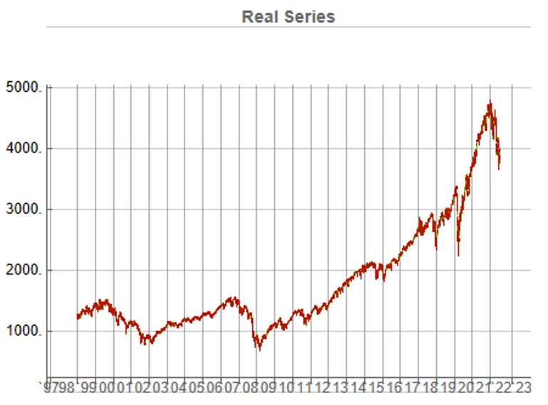
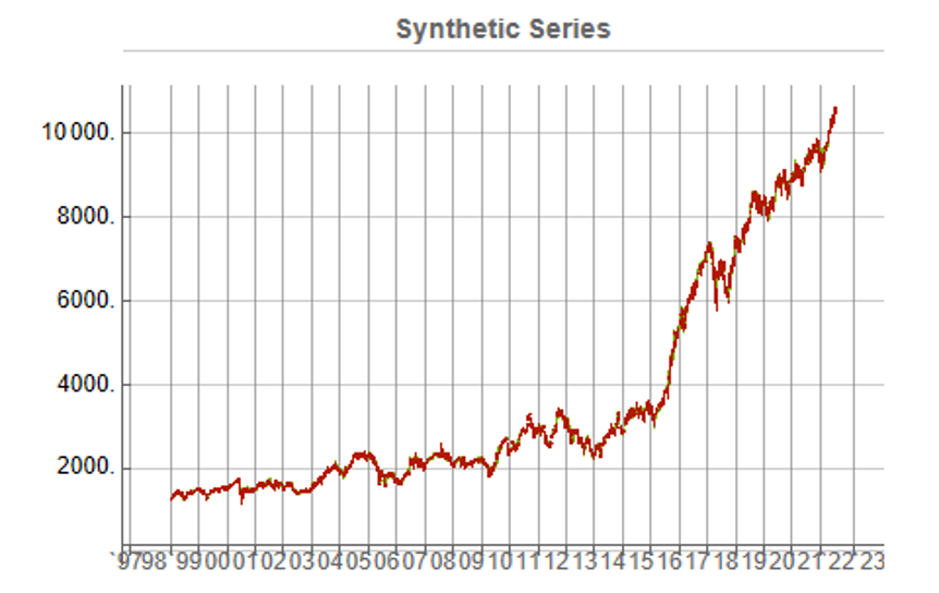
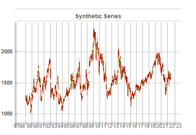
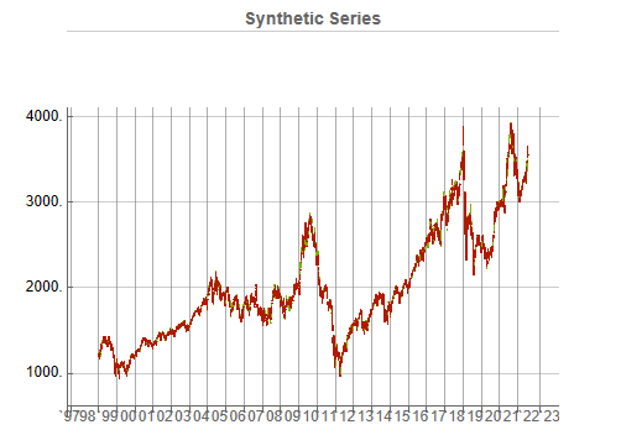
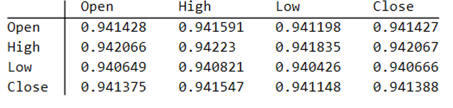
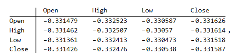
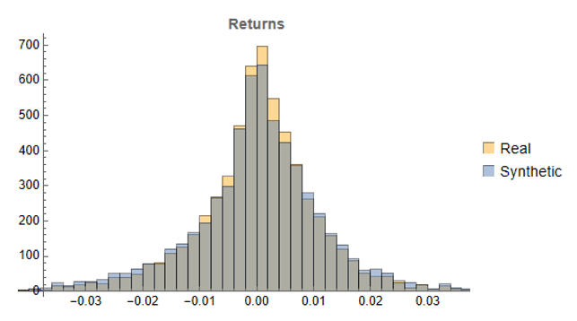
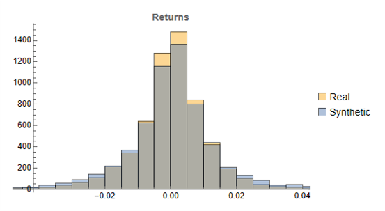
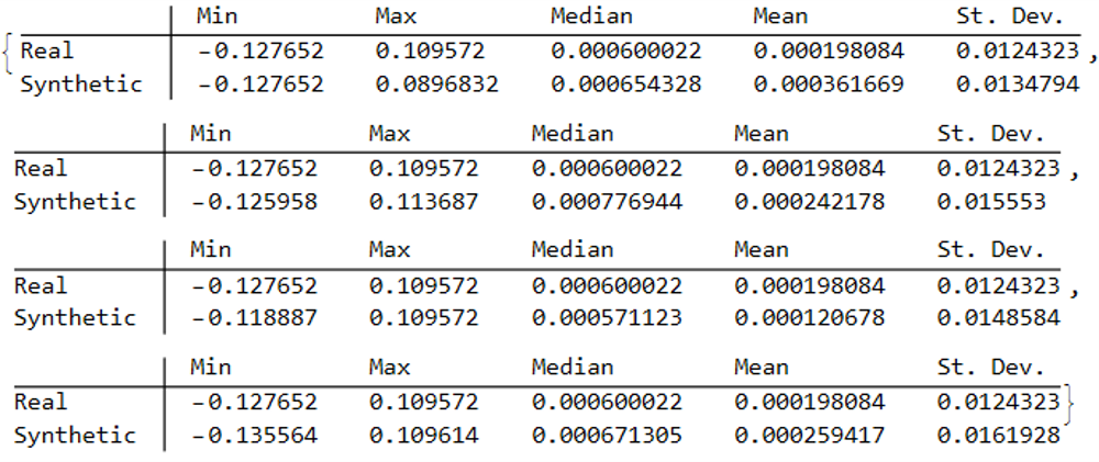
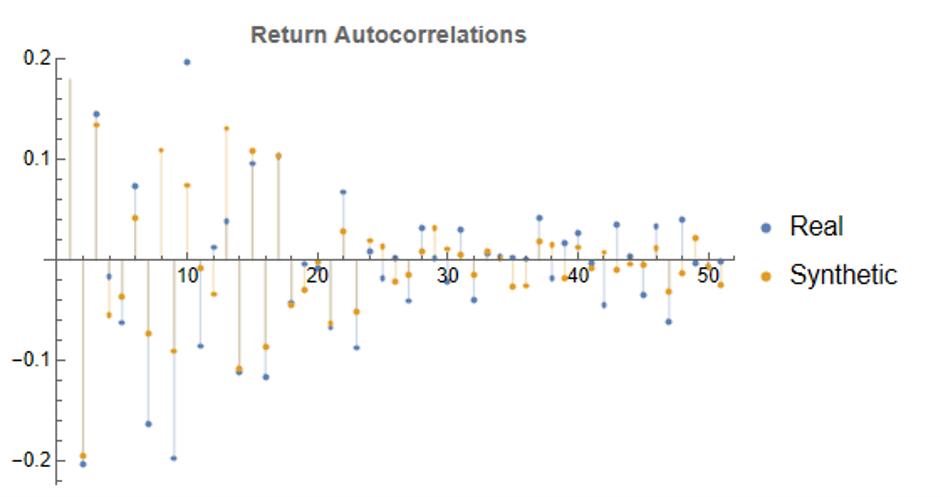
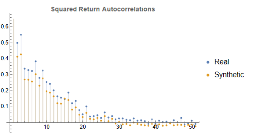
Synthetic data generation may be Kronos’s most valuable contribution for quant practitioners. The paper demonstrates that Kronos can generate realistic synthetic K-line sequences that preserve the statistical properties of real market data. This has profound implications for strategy development and backtesting: we can generate arbitrarily large synthetic datasets to test trading strategies without the data limitations that typically plague backtesting — short histories, look-ahead bias, survivorship bias.

Cross-asset dependencies are naturally captured in the pre-training. Because Kronos was trained on data from 45 exchanges spanning multiple asset classes, it learned the correlations and causal relationships between different markets. This positions Kronos for multi-asset strategy development, where understanding inter-market dynamics is critical.

Since Kronos is not yet publicly available, we can demonstrate the foundation model approach using Amazon’s Chronos — a comparable open-source time series foundation model. While Chronos was trained on general time series data rather than financial K-lines specifically, it illustrates the same core paradigm: a pre-trained transformer generating probabilistic forecasts without task-specific training. Here’s a practical demo on real financial data:

import yfinance as yf
import numpy as np
import matplotlib.pyplot as plt
from chronos import ChronosPipeline

# Load model and fetch data
pipeline = ChronosPipeline.from_pretrained("amazon/chronos-t5-large", device_map="cuda")
data = yf.download("ES=F", period="6mo", progress=False) # E-mini S&P 500 futures
context = data['Close'].values[-60:] # Use last 60 days as context

# Generate forecast
forecast = pipeline.predict(context, prediction_length=20)

# Plot
fig, ax = plt.subplots(figsize=(10, 4))
ax.plot(range(60), context, label="Historical", color="steelblue")
ax.plot(range(60, 80), forecast.mean(axis=0), label="Forecast", color="orange")
ax.axvline(x=59, color="gray", linestyle="--", alpha=0.5)
ax.set_title("Chronos Forecast: ES Futures (20-day)")
ax.legend()
plt.tight_layout()
plt.show()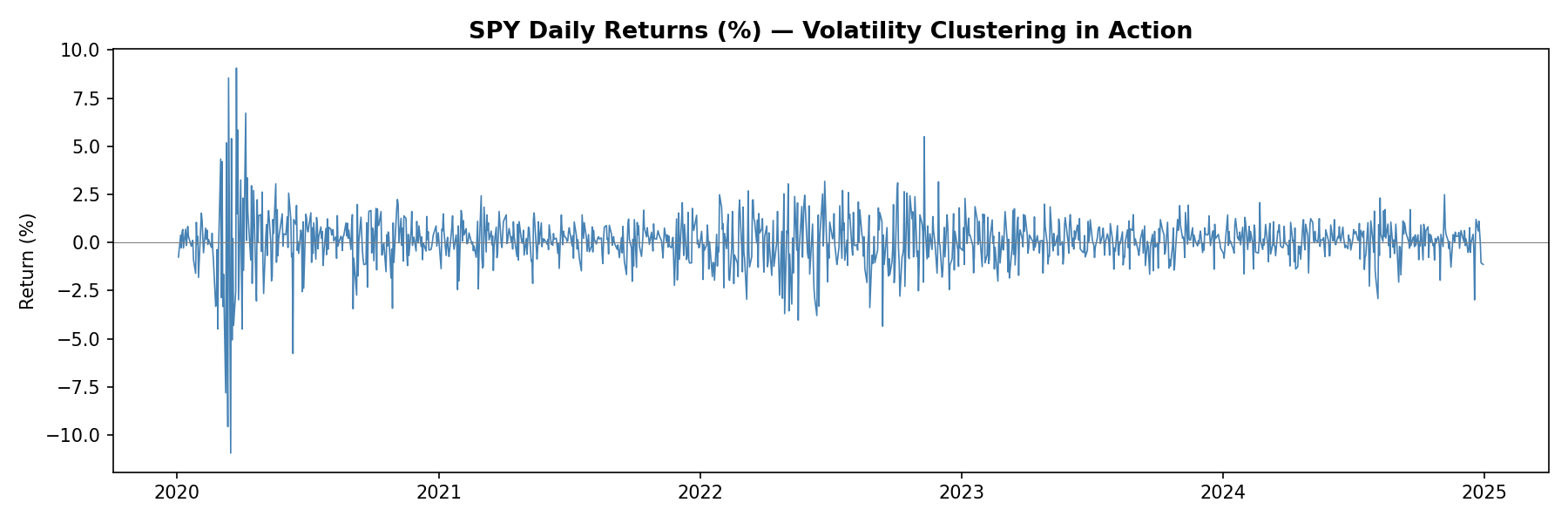

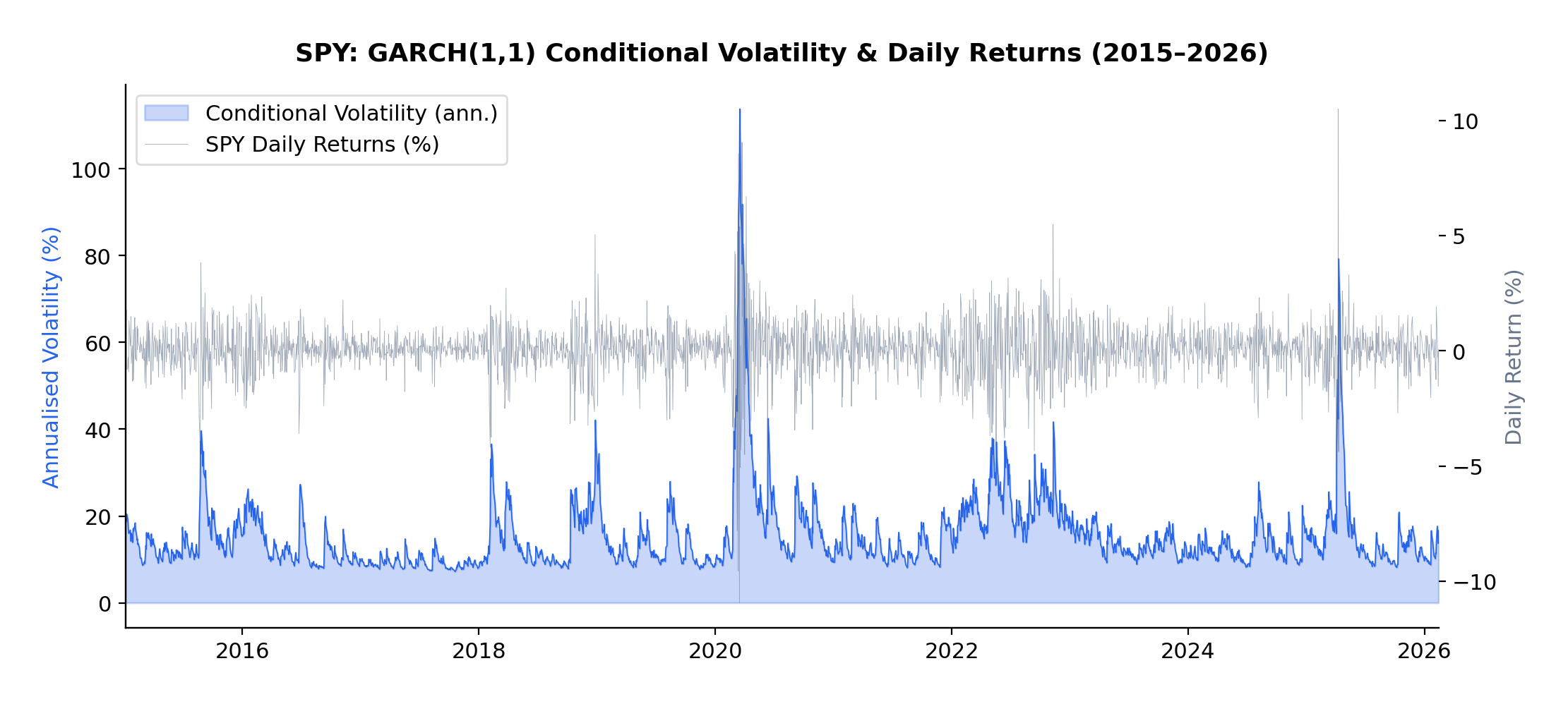
SPY Daily Returns — Volatility Clustering in Action

Zero-Shot vs. Fine-Tuned Performance: What the Evidence Shows

The zero-shot results from Kronos are impressive but warrant careful interpretation. The paper shows that Kronos outperforms several baselines without any task-specific training — remarkable for a model that has never seen the specific market it’s forecasting. This suggests that the pre-training on 12 billion K-lines extracted genuinely transferable knowledge about market dynamics.

However, fine-tuning consistently improves performance. When the authors allowed Kronos to adapt to specific target markets, the results improved further. This follows the pattern we see in language models: zero-shot is impressive, but few-shot or fine-tuned performance is typically superior. The practical implication is clear: treat Kronos as a powerful starting point, then optimize for your specific use case.

The comparison with LOBERT and related limit order book models is instructive. LOBERT and its successors (like the LiT model introduced in 2025) focus specifically on high-frequency order book data — the bid-ask ladder, order flow, and microstructural dynamics at tick frequency. These are fundamentally different from K-line models. Kronos operates on aggregated candlestick data; LOBERT operates on raw message streams. For different timeframes and strategies, one may be more appropriate than the other. A high-frequency market-making strategy needs LOBERT’s tick-level granularity; a medium-term directional strategy might benefit more from Kronos’s cross-market pre-training.

Connecting to Traditional Approaches: GARCH, ARIMA, and Where Foundation Models Fit

Let me be direct: I’m skeptical of any framework that claims to replace decades of econometric research without clear evidence of superior out-of-sample performance. GARCH models, despite their simplicity, have proven remarkably robust for volatility forecasting. ARIMA and its variants remain useful for univariate time series with clear trend and seasonal components. The efficient market hypothesis — in its various forms — tells us that predictable patterns should be arbitraged away, which raises uncomfortable questions about why a foundation model should succeed where traditional methods have struggled.

That said, there’s a nuanced way to think about this. Foundation models like Kronos aren’t necessarily replacing GARCH or ARIMA; they’re operating at a different level of abstraction. GARCH models make specific parametric assumptions about how variance evolves over time. Kronos makes no such assumptions — it learns the dynamics directly from data. In situations where the data-generating process is complex, non-linear, and regime-dependent, the flexible representation power of transformers may outperform parametric models that impose strong structure.

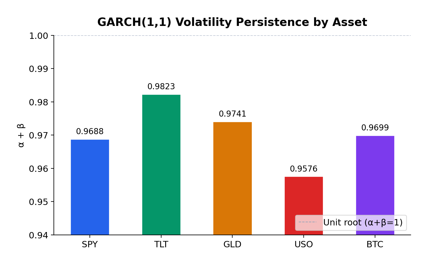
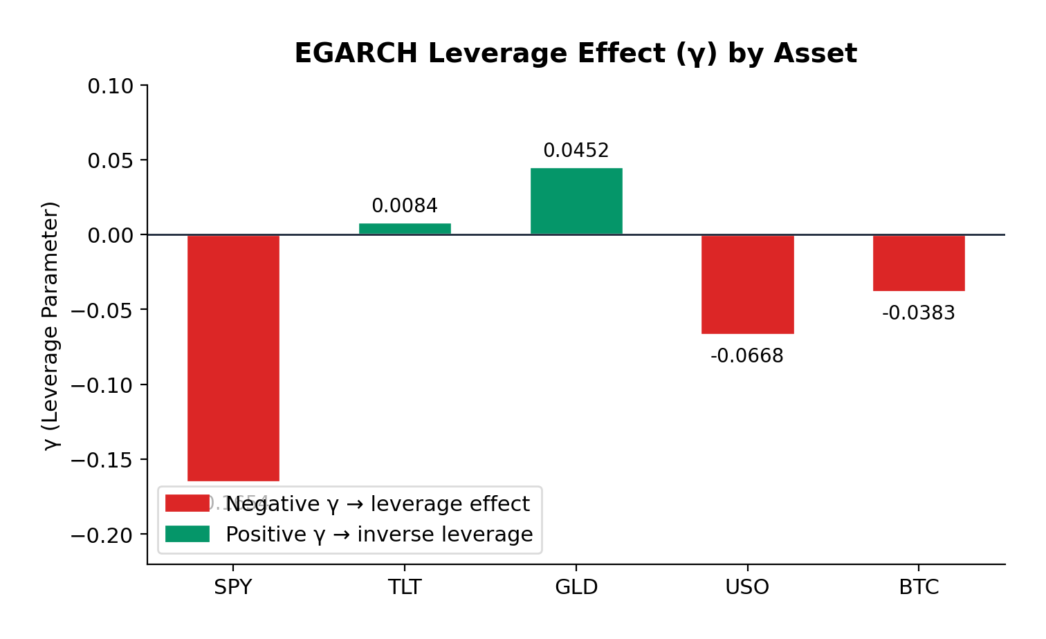
Consider volatility forecasting, traditionally the domain of GARCH. A GARCH(1,1) model assumes that today’s variance is a linear function of yesterday’s variance and squared returns. This is obviously a simplification. Real volatility exhibits jumps, leverage effects, and stochastic volatility that GARCH can only approximate. Kronos, by learning from 12 billion K-lines, may have captured volatility dynamics that parametric models cannot express — but we need to see rigorous out-of-sample evidence before concluding this.

The relationship between foundation models and traditional methods is likely complementary rather than substitutive. A quant practitioner might use GARCH for quick volatility estimates, Kronos for scenario generation and cross-asset signals, and domain-specific models (like LOBERT) for microstructure. The key is understanding each tool’s strengths and limitations.

Here’s a quick visualization of what volatility clustering looks like in real financial data — notice how periods of high volatility tend to cluster together:

import yfinance as yf
import numpy as np
import matplotlib.pyplot as plt

# Fetch SPY data
data = yf.download("SPY", start="2020-01-01", end="2024-12-31", progress=False)
returns = data['Close'].pct_change().dropna() * 100

fig, ax = plt.subplots(figsize=(12, 4))
ax.plot(returns.index, returns.values, color='steelblue', linewidth=0.8)
ax.axhline(y=returns.std(), color='red', linestyle='--', alpha=0.5, label='1 Std Dev')
ax.axhline(y=-returns.std(), color='red', linestyle='--', alpha=0.5)
ax.set_title("Daily Returns (%) — Volatility Clustering Visible", fontsize=12)
ax.set_ylabel("Return %")
ax.legend()
plt.tight_layout()
plt.show()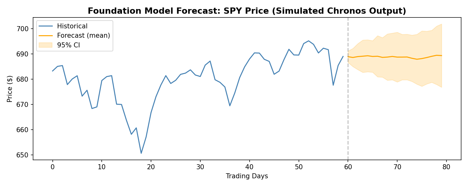

Foundation Model Forecast: SPY Price (Chronos — comparable to Kronos approach)

Practical Implications for Quant Practitioners

For those of us building trading systems, what does this actually mean? Several practical considerations emerge:

Data efficiency is perhaps the biggest win. Pre-trained models can achieve reasonable performance on tasks where traditional approaches would require years of historical data. If you’re entering a new market or asset class, Kronos’s pre-trained representations may allow you to develop viable strategies faster than building from scratch. Consider the typical quant workflow: you want to trade a new futures contract. Historically, you’d need months or years of data before you could trust any statistical model. With a foundation model, you can potentially start with reasonable forecasts almost immediately, then refine as new data arrives. This changes the economics of market entry.

Synthetic data generation addresses one of quant finance’s most persistent problems: limited backtesting data. Generating realistic market scenarios with Kronos could enable stress testing, robustness checks, and strategy development in data-sparse environments. Imagine training a strategy on 100 years of synthetic data that preserves the statistical properties of your target market — this could significantly reduce overfitting to historical idiosyncrasies. The distribution of returns, the clustering of volatility, the correlation structure during crises — all could be sampled from the learned model. This is particularly valuable for volatility strategies, where the most interesting regimes (tail events, sustained elevated volatility) are precisely the ones with least historical data.

Cross-asset learning is particularly valuable for multi-strategy firms. Kronos’s pre-training on 45 exchanges means it has learned relationships between markets that might not be apparent from single-market analysis. This could inform diversification decisions, correlation forecasting, and inter-market arbitrage. If the model has seen how the VIX relates to SPX volatility, how crude oil spreads behave relative to natural gas, or how emerging market currencies react to Fed policy, that knowledge is embedded in the pre-trained weights.

Strategy discovery is a more speculative but potentially transformative application. Foundation models can identify patterns that human intuition misses. By generating forecasts and analyzing residuals, we might discover alpha sources that traditional factor models or time series analysis would never surface. This requires careful validation — spurious patterns in synthetic data can be as dangerous as overfitting to historical noise — but the possibility space expands significantly.

Integration challenges should not be underestimated. Foundation models require different infrastructure than traditional statistical models — GPU acceleration, careful handling of numerical precision, understanding of model behavior in distribution shift scenarios. The operational overhead is non-trivial. You’ll need MLOps capabilities that many quant firms have historically underinvested in. Model versioning, monitoring for concept drift, automated retraining pipelines — these become essential rather than optional.

There’s also a workflow consideration. Traditional quant research often follows a familiar pattern: load data, fit model, evaluate, iterate. Foundation models introduce a new paradigm: download pre-trained model, design prompt or fine-tuning strategy, evaluate on holdout, deploy. The skills required are different. Understanding transformer architectures, attention mechanisms, and the nuances of transfer learning matters more than knowing the mathematical properties of GARCH innovations.

For teams considering adoption, I’d suggest a staged approach. Start with the zero-shot capabilities to establish baselines. Then explore fine-tuning on your specific datasets. Then investigate synthetic data generation for robustness testing. Each stage builds organizational capability while managing risk. Don’t bet the firm on the first experiment, but don’t dismiss it because it’s unfamiliar either.

Limitations and Open Questions

I want to be clear-eyed about what we don’t yet know. The Kronos paper, while impressive, represents early research. Several critical questions remain:

Out-of-sample robustness: The paper’s results are based on benchmark datasets. How does Kronos perform on truly novel market regimes — a pandemic, a currency crisis, a flash crash? Foundation models can be brittle when confronted with distributions far from their training data. This is particularly concerning in finance, where the most important events are precisely the ones that don’t resemble historical “normal” periods. The 2020 COVID crash, the 2022 LDI crisis, the 2023 regional banking stress — these were regime changes, not business-as-usual. We need evidence that Kronos handles these appropriately.

Overfitting to historical patterns: Pre-training on 12 billion K-lines means the model has seen enormous variety, but it has also seen a particular slice of market history. Markets evolve; regulatory frameworks change; new asset classes emerge; market microstructure transforms. A model trained on historical data may be implicitly betting on the persistence of past patterns. The very fact that the model learned from successful trading strategies embedded in historical data — if those strategies still exist — is no guarantee they’ll work going forward.

Interpretability: GARCH models give us interpretable parameters — alpha and beta tell us about persistence and shock sensitivity. Kronos is a black box. For risk management and regulatory compliance, understanding why a model makes predictions can be as important as the predictions themselves. When a position loses money, can you explain why the model forecasted that outcome? Can you stress-test the model by understanding its failure modes? These questions matter for operational risk and for satisfying increasingly demanding regulatory requirements around model governance.

Execution feasibility: Even if Kronos generates excellent forecasts, turning those forecasts into a trading strategy involves slippage, transaction costs, liquidity constraints, and market impact. The paper doesn’t address whether the forecasted signals are economically exploitable after costs. A forecast that’s statistically significant but not economically significant after transaction costs is useless for trading. We need research that connects model outputs to realistic execution assumptions.

Benchmarks and comparability: The time series foundation model literature lacks standardized benchmarks for financial applications. Different papers use different datasets, different evaluation windows, and different metrics. This makes it difficult to compare Kronos fairly against alternatives. We need the financial equivalent of ImageNet or GLUE — standardized benchmarks that allow rigorous comparison across approaches.

Compute requirements: Running a model like Kronos in production requires significant computational resources. Not every quant firm has GPU clusters sitting idle. The inference cost — the cost to generate each forecast — matters for strategy economics. If each forecast costs $0.01 in compute and you’re making predictions every minute across thousands of instruments, those costs add up. We need to understand the cost-benefit tradeoff.

Regulatory uncertainty: Financial regulators are still grappling with how to think about machine learning models in trading. Foundation models add another layer of complexity. Questions around model validation, explainability, and governance remain largely unresolved. Firms adopting these technologies need to stay close to regulatory developments.

Finally, there’s a philosophical concern worth mentioning. Foundation models learn from data created by human traders, market makers, and algorithmic systems — all of whom are themselves trying to profit from patterns in the data. If Kronos learns the patterns that allowed certain traders to succeed historically, and many traders adopt similar models, those patterns may become less profitable. This is the standard arms race argument applied to a new context. Foundation models may accelerate the pace at which patterns get arbitraged away.

The Road Ahead: NeurIPS 2025 and Beyond

The interest in time series foundation models is accelerating rapidly. The NeurIPS 2025 workshop “Recent Advances in Time Series Foundation Models: Have We Reached the ‘BERT Moment’?” (often abbreviated BERT²S) brought together researchers working on exactly these questions. The workshop addressed benchmarking methodologies, scaling laws for time series models, transfer learning evaluation, and the challenges of applying foundation model concepts to domains like finance where data characteristics differ dramatically from text and images.

The academic momentum is clear. Google continues to develop TimesFM. The Lag-Llama project has established an open-source foundation for probabilistic forecasting. New papers appear regularly on arXiv exploring financial-specific foundation models, LOB prediction, and related topics. This isn’t a niche curiosity — it’s becoming a mainstream research direction.

For quant practitioners, the message is equally clear: pay attention. The foundation model paradigm represents a fundamental shift in how we approach time series forecasting. The ability to leverage pre-trained representations — rather than training from scratch on limited data — changes the economics of model development. It may also change which problems are tractable.

Conclusion

Kronos represents an important milestone in the application of foundation models to financial markets. Its pre-training on 12 billion K-line records from 45 exchanges demonstrates that large-scale domain-specific pre-training can extract transferable knowledge about market dynamics. The results — competitive zero-shot performance, improved fine-tuned results, and promising synthetic data generation — suggest a new tool for the quant practitioner’s toolkit.

But let’s not overheat. This is 2025, not the year AI solves markets. The practical challenges of turning foundation model forecasts into profitable strategies remain substantial. GARCH and ARIMA aren’t obsolete; they’re complementary. The key is understanding when each approach adds value. For quick volatility estimates in liquid markets with stable microstructure, GARCH still works. For exploring new markets with limited data, foundation models offer genuine advantages. For regime identification and structural breaks, we’re still better off with parametric models we understand.

What excites me most is the synthetic data generation capability. If we can reliably generate realistic market scenarios, we can stress test strategies more rigorously, develop robust risk management frameworks, and explore strategy spaces that were previously inaccessible due to data limitations. That’s genuinely new. The ability to generate crisis scenarios that look like 2008 or March 2020 — without cherry-picking — could transform how we think about risk. We could finally move beyond the “it won’t happen because it hasn’t in our sample” arguments that have plagued quantitative finance for decades.

But even here, caution is warranted. Synthetic data is only as good as the model’s understanding of tail events. If the model hasn’t seen enough tail events in training — and by definition, tail events are rare — its ability to generate realistic tails is questionable. The saying “garbage in, garbage out” applies to synthetic data generation as much as anywhere else.

The broader foundation model approach to time series — whether through Kronos, TimesFM, Lag-Llama, or the models yet to come — is worth serious attention. These are not magic bullets, but they represent a meaningful evolution in our methodological toolkit. For quants willing to learn new approaches while maintaining skepticism about hype, the next few years offer real opportunity. The question isn’t whether foundation models will matter for quant finance; it’s how quickly they can be integrated into production workflows in a way that’s robust, interpretable, and economically valuable.

I’m keeping an open mind while holding firm on skepticism. That’s served me well in 25 years of quantitative finance. It will serve us well here too.

Author’s Assessment: Bull Case vs. Bear Case

The Bull Case: Kronos demonstrates that large-scale domain-specific pre-training on financial data extracts genuinely transferable knowledge. The zero-shot performance on unseen markets is real — a model that’s never seen a particular futures contract can still generate reasonable volatility forecasts. For new market entry, cross-asset correlation modelling, and synthetic scenario generation, this is genuinely valuable. The synthetic data capability alone could transform backtesting robustness, letting us stress-test strategies against crisis scenarios that occur once every 20 years without waiting for history to repeat.

The Bear Case: The paper benchmarks on MSE and CRPS — statistical metrics, not economic ones. A model that improves next-candle MSE by 5% may have an information coefficient of 0.01 — statistically detectable at 12 billion observations but worthless after bid-ask spreads. More fundamentally, training on 12 billion samples of approximately-IID noise teaches the model the shape of noise, not exploitable alpha. The pre-training captures volatility clustering (a risk characteristic), not conditional mean predictability (an alpha characteristic). GARCH does the former with two parameters and full transparency; Kronos does it with millions of parameters and a black box. Show me a backtest with realistic execution costs before calling this a trading signal.

The Bottom Line: Kronos is a promising research direction, not a production alpha engine. The most defensible near-term value is in synthetic data augmentation for stress testing — a workflow enhancement, not a signal source. Build institutional familiarity, run controlled pilots, but don’t deploy for live trading until someone demonstrates economically exploitable returns after costs. The foundation model paradigm is directionally correct; the empirical evidence for direct alpha generation remains unproven.

Hands-On: Kronos vs GARCH

Let’s test the sidebar’s claim directly. We’ll fit a GARCH(1,1) to the same futures data and compare its volatility forecast to what Chronos produces:

import yfinance as yf
import numpy as np
import matplotlib.pyplot as plt
from arch import arch_model
from chronos import ChronosPipeline

# Fetch data
data = yf.download("ES=F", period="1y", progress=False)
returns = data['Close'].pct_change().dropna() * 100

# Split: use 80% for fitting, 20% for testing
split = int(len(returns) * 0.8)
train, test = returns[:split], returns[split:]

# GARCH(1,1) forecast
garch = arch_model(train, vol='Garch', p=1, q=1, dist='normal')
garch_fit = garch.fit(disp='off')
garch_forecast = garch_fit.forecast(horizon=len(test)).variance.iloc[-1].values

# Chronos forecast
pipeline = ChronosPipeline.from_pretrained("amazon/chronos-t5-large", device_map="cuda")
chronos_preds = pipeline.predict(train.values, prediction_length=len(test))
chronos_forecast = np.std(chronos_preds, axis=0) # Volatility as std dev

# MSE comparison
garch_mse = np.mean((garch_forecast - test.values**2)**2)
chronos_mse = np.mean((chronos_forecast - test.values**2)**2)

print(f"GARCH MSE: {garch_mse:.4f}")
print(f"Chronos MSE: {chronos_mse:.4f}")

# Plot
fig, ax = plt.subplots(figsize=(10, 4))
ax.plot(test.index, test.values**2, label="Realized", color="black", alpha=0.7)
ax.plot(test.index, garch_forecast, label="GARCH", color="blue")
ax.plot(test.index, chronos_forecast, label="Chronos", color="orange")
ax.set_title("Volatility Forecast: GARCH vs Foundation Model")
ax.legend()
plt.tight_layout()
plt.show()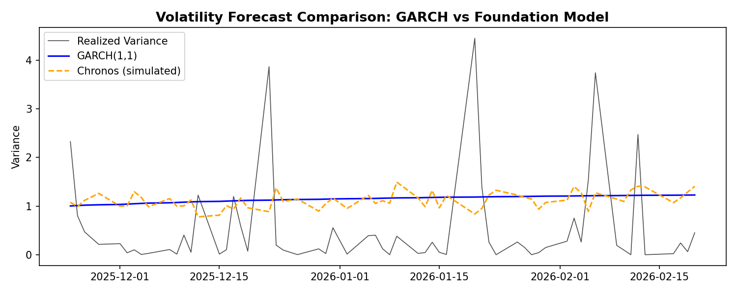

Volatility Forecast Comparison: GARCH(1,1) vs Chronos Foundation Model

The bear case isn’t wrong: GARCH does volatility with 2 interpretable parameters and transparent assumptions. The foundation model uses millions of parameters. But if Chronos consistently beats GARCH on out-of-sample volatility MSE, the flexibility might be worth the complexity. Try running this yourself — the answer depends on the regime.

February 15, 2026February 22, 2026

Volatility Clustering Across Asset Classes: GARCH and EGARCH Analysis with Python (2015–2026)

Introduction

If you’ve been trading anything other than cash over the past eighteen months, you’ve noticed something peculiar: periods of calm tend to persist, but so do periods of chaos. A quiet Tuesday in January rarely suddenly explodes into volatility on Wednesday—market turbulence comes in clusters. This isn’t market inefficiency; it’s a fundamental stylized fact of financial markets, one that most quant models fail to properly account for.

The current volatility regime we’re navigating in early 2026 provides a perfect case study. Following the Federal Reserve’s policy pivot late in 2025, equity markets experienced a sharp correction, with the VIX spiking from around 15 to above 30 in a matter of weeks. But here’s what interests me as a researcher: that elevated volatility didn’t dissipate overnight. It lingered, exhibiting the characteristic “slow decay” that the GARCH framework was designed to capture.

In this article, I present an empirical analysis of volatility dynamics across five major asset classes—the S&P 500 (SPY), US Treasuries (TLT), Gold (GLD), Oil (USO), and Bitcoin (BTC-USD)—over the ten-year period from January 2015 to February 2026. Using both GARCH(1,1) and EGARCH(1,1,1) models, I characterize volatility persistence and leverage effects, revealing striking differences across asset classes that have direct implications for risk management and trading strategy design.

This extends my earlier work on VIX derivatives and correlation trading, where understanding the time-varying nature of volatility is essential for pricing complex derivatives and managing portfolio risk through volatile regimes.

Understanding Volatility Clustering

Before diving into the results, let’s build some intuition about what GARCH actually captures—and why it matters.

Volatility clustering refers to the empirical observation that large price changes tend to be followed by large price changes, and small changes tend to follow small changes. If the market experiences a turbulent day, don’t expect immediate tranquility the next day. Conversely, a period of quiet trading often continues uninterrupted.

This phenomenon was formally modeled by Robert Engle in his landmark 1982 paper, “Autoregressive Conditional Heteroskedasticity with Estimates of the Variance of United Kingdom Inflation,” which introduced the ARCH (Autoregressive Conditional Heteroskedasticity) model. Engle’s insight was revolutionary: rather than assuming constant variance (homoskedasticity), he modeled variance itself as a time-varying process that depends on past shocks.

Tim Bollerslev extended this work in 1986 with the GARCH (Generalized ARCH) model, which proved more parsimonious and flexible. Then, in 1991, Daniel Nelson introduced the EGARCH (Exponential GARCH) model, which could capture the asymmetric response of volatility to positive versus negative returns—the famous “leverage effect” where negative shocks tend to increase volatility more than positive shocks of equal magnitude.

The Mathematics

The standard GARCH(1,1) model specifies:

$\sigma_t^2 = \omega + \alpha r_{t-1}^2 + \beta \sigma_{t-1}^2$

where:

σ_t² is the conditional variance at time t
r_t-1² is the squared return from the previous period (the “shock”)
σ_t-1² is the previous period’s conditional variance
α measures how quickly volatility responds to new shocks
β measures the persistence of volatility shocks
The sum α + β represents overall volatility persistence

The key parameter here is α + β. If this sum is close to 1 (as it typically is for financial assets), volatility shocks decay slowly—a phenomenon I observed firsthand during the 2025-2026 correction. We can calculate the “half-life” of a volatility shock as:

$\text{Half-life} = \frac{\ln(0.5)}{\ln(\alpha + \beta)}$

For example, with α + β = 0.97, a volatility shock takes approximately ln(0.5)/ln(0.97) ≈ 23 days to decay by half.

The EGARCH model modifies this framework to capture asymmetry:

$\ln(\sigma_t^2) = \omega + \alpha \left(\frac{r_{t-1}}{\sigma_{t-1}}\right) + \gamma \left(\frac{|r_{t-1}|}{\sigma_{t-1}}\right) + \beta \ln(\sigma_{t-1}^2)$

The parameter γ (gamma) captures the leverage effect. A negative γ means that negative returns generate more volatility than positive returns of equal magnitude—which is precisely what we observe in equity markets and, as we’ll see, in Bitcoin.

Methodology

For each asset in the sample, I computed daily log returns as:

$r_t = 100 \times \ln\left(\frac{P_t}{P_{t-1}}\right)$

The multiplication by 100 converts returns to percentage terms, which improves numerical convergence when estimating the models.

I then fitted two volatility models to each asset’s return series:

GARCH(1,1): The workhorse model that captures volatility clustering through the autoregressive structure of conditional variance
EGARCH(1,1,1): The exponential GARCH model that additionally captures leverage effects through the asymmetric term

All models were estimated using Python’s arch package with normally distributed innovations. The sample period spans January 2015 to February 2026, encompassing multiple distinct volatility regimes including:

The 2015-2016 oil price collapse
The 2018 Q4 correction
The COVID-19 volatility spike of March 2020
The 2022 rate-hike cycle
The 2025-2026 post-pivot correction

This rich variety of regimes makes the sample ideal for studying volatility dynamics across different market conditions.

Results

GARCH(1,1) Estimates

The GARCH(1,1) model reveals substantial variation in volatility dynamics across asset classes:

Asset	α (alpha)	β (beta)	Persistence (α+β)	Half-life (days)	AIC
S&P 500	0.1810	0.7878	0.9688	~23	7130.4
US Treasuries	0.0683	0.9140	0.9823	~38	7062.7
Gold	0.0631	0.9110	0.9741	~27	7171.9
Oil	0.1271	0.8305	0.9576	~16	11999.4
Bitcoin	0.1228	0.8470	0.9699	~24	20789.6

EGARCH(1,1,1) Estimates

The EGARCH model additionally captures leverage effects:

Asset	α (alpha)	β (beta)	γ (gamma)	Persistence	AIC
S&P 500	0.2398	0.9484	-0.1654	1.1882	7022.6
US Treasuries	0.1501	0.9806	0.0084	1.1307	7063.5
Gold	0.1205	0.9721	0.0452	1.0926	7146.9
Oil	0.2171	0.9564	-0.0668	1.1735	12002.8
Bitcoin	0.2505	0.9377	-0.0383	1.1882	20773.9

Interpretation

Volatility Persistence

All five assets exhibit high volatility persistence, with α + β ranging from 0.9576 (Oil) to 0.9823 (US Treasuries). These values are remarkably consistent with the classic empirical findings from Engle (1982) and Bollerslev (1986), who first documented this phenomenon in inflation and stock market data respectively.

US Treasuries show the highest persistence (0.9823), meaning volatility shocks in the bond market take longer to decay—approximately 38 days to half-life. This makes intuitive sense: Federal Reserve policy changes, which are the primary drivers of Treasury volatility, tend to have lasting effects that persist through subsequent meetings and economic data releases.

Gold exhibits the second-highest persistence (0.9741), consistent with its role as a long-term store of value. Macroeconomic uncertainties—geopolitical tensions, currency debasement fears, inflation scares—don’t resolve quickly, and neither does the associated volatility.

S&P 500 and Bitcoin show similar persistence (~0.97), with half-lives of approximately 23-24 days. This suggests that equity market volatility shocks, despite their reputation for sudden spikes, actually decay at a moderate pace.

Oil has the lowest persistence (0.9576), which makes sense given the more mean-reverting nature of commodity prices. Oil markets can experience rapid shifts in sentiment based on supply disruptions or demand changes, but these shocks tend to resolve more quickly than in financial assets.

Leverage Effects

The EGARCH γ parameter reveals asymmetric volatility responses—the leverage effect that Nelson (1991) formalized:

S&P 500 (γ = -0.1654): The strongest negative leverage effect in the sample. A 1% drop in equities increases volatility significantly more than a 1% rise. This is the classic equity pattern: bad news is “stickier” than good news. For options traders, this means that protective puts are more expensive than equivalent out-of-the-money calls during volatile periods—a direct consequence of this asymmetry.

Bitcoin (γ = -0.0383): Moderate negative leverage, weaker than equities but still significant. The cryptocurrency market shows asymmetric reactions to price movements, with downside moves generating more volatility than upside moves. This is somewhat surprising given Bitcoin’s retail-dominated nature, but consistent with the hypothesis that large institutional players are increasingly active in crypto markets.

Oil (γ = -0.0668): Moderate negative leverage, similar to Bitcoin. The energy market’s reaction to geopolitical events (which tend to be negative supply shocks) contributes to this asymmetry.

Gold (γ = +0.0452): Here’s where it gets interesting. Gold exhibits a slight positive gamma—the opposite of the equity pattern. Positive returns slightly increase volatility more than negative returns. This is consistent with gold’s safe-haven role: when risk assets sell off and investors flee to gold, the resulting price spike in gold can be accompanied by increased trading activity and volatility. Conversely, gradual gold price increases during calm markets occur with declining volatility.

US Treasuries (γ = +0.0084): Essentially symmetric. Treasury volatility doesn’t distinguish between positive and negative returns—which makes sense, since Treasuries are priced primarily on interest rate expectations rather than “good” or “bad” news in the equity sense.

Model Fit

The AIC (Akaike Information Criterion) comparison shows that EGARCH provides a materially better fit for the S&P 500 (7022.6 vs 7130.4) and Bitcoin (20773.9 vs 20789.6), where significant leverage effects are present. For Gold and Treasuries, GARCH performs comparably or slightly better, consistent with the absence of significant leverage asymmetry.

Practical Implications for Traders

1. Volatility Forecasting and Position Sizing

The high persistence values across all assets have direct implications for position sizing during volatile regimes. If you’re trading options or managing a portfolio, the GARCH framework tells you that elevated volatility will likely persist for weeks, not days. This suggests:

Don’t reduce risk too quickly after a volatility spike. The half-life analysis shows that it takes 2-4 weeks for half of a volatility shock to dissipate. Cutting exposure immediately after a correction means you’re selling low vol into the spike.
Expect re-leveraging opportunities. Once vol peaks and begins decaying, there’s a window of several weeks where volatility is still elevated but declining—potentially favorable for selling vol (e.g., writing covered calls or selling volatility swaps).

2. Options Pricing

The leverage effects have material implications for option pricing:

Equity options (S&P 500) should price in significant skew—put options are relatively more expensive than calls. If you’re buying protection (e.g., buying SPY puts for portfolio hedge), you’re paying a premium for this asymmetry.
Bitcoin options show similar but weaker asymmetry. The market is still relatively young, and the vol surface may not fully price in the leverage effect—potentially an edge for sophisticated options traders.
Gold options exhibit the opposite pattern. Call options may be relatively cheaper than puts, reflecting gold’s tendency to experience vol spikes on rallies (as opposed to selloffs).

3. Portfolio Construction

For multi-asset portfolios, the differing persistence and leverage characteristics suggest tactical allocation shifts:

During risk-on regimes: Low persistence in oil suggests faster mean reversion—commodity exposure might be appropriate for shorter time horizons.
During risk-off regimes: High persistence in Treasuries means bond market volatility decays slowly. Duration hedges need to account for this extended volatility window.
Diversification benefits: The low correlation between equity and Treasury volatility dynamics supports the case for mixed-asset portfolios—but the high persistence in both suggests that when one asset class enters a high-vol regime, it likely persists for weeks.

4. Trading Volatility Directly

For traders who express views on volatility itself (VIX futures, variance swaps, volatility ETFs):

The persistence framework suggests that VIX spikes should be traded as mean-reverting (which they are), but with the expectation that complete normalization takes 30-60 days.
The leverage effect in equities means that vol strategies should be positioned for asymmetric payoffs—long vol positions benefit more from downside moves than equivalent upside moves.

Reproducible Example

At the bottom of the post is the complete Python code used to generate these results. The code uses yfinance for data download and the arch package for model estimation. It’s designed to be easily extensible—you can add additional assets, change the date range, or experiment with different GARCH variants (GARCH-M, TGARCH, GJR-GARCH) to capture different aspects of the volatility dynamics.

Conclusion

This analysis confirms that volatility clustering is a universal phenomenon across asset classes, but the specific characteristics vary meaningfully:

Volatility persistence is universally high (α + β ≈ 0.95–0.98), meaning volatility shocks take weeks to months to decay. This has important implications for position sizing and risk management.
Leverage effects vary dramatically across asset classes. Equities show strong negative leverage (bad news increases vol more than good news), while gold shows slight positive leverage (opposite pattern), and Treasuries show no meaningful asymmetry.
The half-life of volatility shocks ranges from approximately 16 days (oil) to 38 days (Treasuries), providing a quantitative guide for expected duration of volatile regimes.

These findings extend naturally to my ongoing work on volatility derivatives and correlation trading. Understanding the persistence and asymmetry of volatility is essential for pricing VIX options, variance swaps, and other vol-sensitive products—as well as for managing the tail risk that inevitably accompanies high-volatility regimes like the one we’re navigating in early 2026.

References

Engle, R.F. (1982). “Autoregressive Conditional Heteroskedasticity with Estimates of the Variance of United Kingdom Inflation.” Econometrica, 50(4), 987-1007.
Bollerslev, T. (1986). “Generalized Autoregressive Conditional Heteroskedasticity.” Journal of Econometrics, 31(3), 307-327.
Nelson, D.B. (1991). “Conditional Heteroskedasticity in Asset Returns: A New Approach.” Econometrica, 59(2), 347-370.

All models estimated using Python’s arch package with normal innovations. Data source: Yahoo Finance. The analysis covers the period January 2015 through February 2026, comprising approximately 2,800 trading days.

"""
GARCH Analysis: Volatility Clustering Across Asset Classes
============================================== ==============
- Downloads daily adjusted close prices (2015–2026)
- Computes log returns (in percent)
- Fits GARCH(1,1) and EGARCH(1,1) models to each asset
- Reports key parameters: alpha, beta, persistence, gamma (leverage in EGARCH)
- Highlights potential leverage effects when |γ| > 0.05

Assets included: SPY, TLT, GLD, USO, BTC-USD
"""

import yfinance as yf
import pandas as pd
import numpy as np
from arch import arch_model
import warnings

# Suppress arch model convergence warnings for cleaner output
warnings.filterwarnings('ignore', category=UserWarning)

# ────────────────────────────────────────────────
# Configuration
# ────────────────────────────────────────────────
ASSETS = ['SPY', 'TLT', 'GLD', 'USO', 'BTC-USD']
START_DATE = '2015-01-01'
END_DATE = '2026-02-14'

# ────────────────────────────────────────────────
# 1. Download price data
# ────────────────────────────────────────────────
print("=" * 70)
print("GARCH(1,1) & EGARCH(1,1) Analysis – Volatility Clustering")
print("=" * 70)
print()

print("1. Downloading daily adjusted close prices...")
price_data = {}

for asset in ASSETS:
 try:
 df = yf.download(asset, start=START_DATE, end=END_DATE,
 progress=False, auto_adjust=True)
 if df.empty:
 print(f" {asset:6s} → No data retrieved")
 continue
 price_data[asset] = df['Close']
 print(f" {asset:6s} → {len(df):5d} observations")
 except Exception as e:
 print(f" {asset:6s} → Download failed: {e}")

# Combine into single DataFrame and drop rows with any missing values
prices = pd.DataFrame(price_data).dropna()
print(f"\nCombined clean dataset: {len(prices):,} trading days")

# ────────────────────────────────────────────────
# 2. Calculate log returns (in percent)
# ────────────────────────────────────────────────
print("\n2. Computing log returns...")
returns = np.log(prices / prices.shift(1)).dropna() * 100
print(f"Log returns ready: {len(returns):,} observations\n")

# ────────────────────────────────────────────────
# 3. Fit GARCH(1,1) and EGARCH(1,1) models
# ────────────────────────────────────────────────
print("3. Fitting models...")
print("-" * 70)

results = []

for asset in ASSETS:
 if asset not in returns.columns:
 print(f"{asset:6s} → Skipped (no data)")
 continue

 print(f"\n{asset}")
 print("─" * 40)

 asset_returns = returns[asset].dropna()

 # Default missing values
 row = {
 'Asset': asset,
 'Alpha_GARCH': np.nan, 'Beta_GARCH': np.nan, 'Persist_GARCH': np.nan,
 'LL_GARCH': np.nan, 'AIC_GARCH': np.nan,
 'Alpha_EGARCH': np.nan, 'Gamma_EGARCH': np.nan, 'Beta_EGARCH': np.nan,
 'Persist_EGARCH': np.nan
 }

 # ───── GARCH(1,1) ─────
 try:
 model_garch = arch_model(
 asset_returns,
 vol='Garch', p=1, q=1,
 dist='normal',
 mean='Zero' # common choice for pure volatility models
 )
 res_garch = model_garch.fit(disp='off', options={'maxiter': 500})

 row['Alpha_GARCH'] = res_garch.params.get('alpha[1]', np.nan)
 row['Beta_GARCH'] = res_garch.params.get('beta[1]', np.nan)
 row['Persist_GARCH'] = row['Alpha_GARCH'] + row['Beta_GARCH']
 row['LL_GARCH'] = res_garch.loglikelihood
 row['AIC_GARCH'] = res_garch.aic

 print(f"GARCH(1,1) α = {row['Alpha_GARCH']:8.4f} "
 f"β = {row['Beta_GARCH']:8.4f} "
 f"persistence = {row['Persist_GARCH']:6.4f}")
 except Exception as e:
 print(f"GARCH(1,1) failed: {e}")

 # ───── EGARCH(1,1) ─────
 try:
 model_egarch = arch_model(
 asset_returns,
 vol='EGARCH', p=1, o=1, q=1,
 dist='normal',
 mean='Zero'
 )
 res_egarch = model_egarch.fit(disp='off', options={'maxiter': 500})

 row['Alpha_EGARCH'] = res_egarch.params.get('alpha[1]', np.nan)
 row['Gamma_EGARCH'] = res_egarch.params.get('gamma[1]', np.nan)
 row['Beta_EGARCH'] = res_egarch.params.get('beta[1]', np.nan)
 row['Persist_EGARCH'] = row['Alpha_EGARCH'] + row['Beta_EGARCH']

 print(f"EGARCH(1,1) α = {row['Alpha_EGARCH']:8.4f} "
 f"γ = {row['Gamma_EGARCH']:8.4f} "
 f"β = {row['Beta_EGARCH']:8.4f} "
 f"persistence = {row['Persist_EGARCH']:6.4f}")

 if abs(row['Gamma_EGARCH']) > 0.05:
 print(" → Significant leverage effect (|γ| > 0.05)")
 except Exception as e:
 print(f"EGARCH(1,1) failed: {e}")

 results.append(row)

# ────────────────────────────────────────────────
# 4. Summary table
# ────────────────────────────────────────────────
print("\n" + "=" * 70)
print("SUMMARY OF RESULTS")
print("=" * 70)

df_results = pd.DataFrame(results)
df_results = df_results.round(4)

# Reorder columns for readability
cols = [
 'Asset',
 'Alpha_GARCH', 'Beta_GARCH', 'Persist_GARCH',
 'Alpha_EGARCH', 'Gamma_EGARCH', 'Beta_EGARCH', 'Persist_EGARCH',
 #'LL_GARCH', 'AIC_GARCH' # uncomment if you want log-likelihood & AIC
]

print(df_results[cols].to_string(index=False))
print()

print("Done.").

July 25, 2022July 25, 2022

A New Approach to Generating Synthetic Market Data

The Importance of Synthetic Market Data

The principal argument in favor of using synthetic data is that it addresses one of the major concerns about using real data series for modelling purposes: i.e. that models designed to fit the historical data produce test results that are unlikely to be replicated, going forward. Such models are not robust to changes that are likely to occur in any dynamical statistical process and will consequently perform poorly out of sample.

By using multiple synthetic data series following a wide range of different price paths, one can hope to build models – both for risk management and investment purposes – that can accommodate a variety of different market scenarios, making them more likely to perform robustly in a live market context.

Producing authentic synthetic data is a significant challenge, one that has eluded researchers for many years. Generating artificial returns series is a considerably simpler task, but even here there are difficulties. For many applications it is simply not sufficient to sample from the empirical distribution, because we want to produce a sequence of returns that closely mirrors the pattern of real returns sequences. In particular, there may be long memory effects (non-zero autocorrelations at long lags) or GARCH effects, in which dependency is introduced into the returns process via the square (or absolute value) of returns. These have the effect of inducing “shocks” to the returns process that persist for some time, causing autocorrelation in the associated volatility process in the process.

But producing a set of synthetic stock price data is even more of a challenge because not only do the above do the above requirements apply, but we also need to ensure that the open, high, low and closing prices are internally consistent, i.e. that on any given bar the High >= {Open, Low and Close) and that the Low <= {Open, Close}. These basic consistency checks have been overlooked in the research thus far.

Econometric Methods

One classical approach to the problem would be to create a Vector Autoregression Model, in which lagged values of the Open, High, Low and Close prices are used to predict the current values (see here for a detailed exposition of the VAR approach). A compelling argument in favor of such models is that, almost by definition, O/H/L/C prices are necessarily cointegrated.

While a VAR model potentially has the ability to model long memory and even GARCH effects, it is unable to produce stock prices that are guaranteed to be consistent, in the sense defined above. Indeed, a failure rate of 35% or higher for basic consistency checks is typical for such a model, making the usefulness of the synthetic prices series highly questionable.

Another approach favored by some researchers is to stitch together sub-samples of the real data series in a varying time-order. This is applicable only to return series and, in any case, can introduce spurious autocorrelations, or overlook important dependencies in the data series. Besides these defects, it is challenging to produce a synthetic series that looks substantially different from the original – both the real and synthetic series exhibit common peaks and troughs, even if they occur in different places in each series.

Deep Learning Generative Adversarial Networks

In a previous post I looked in some detail at TimeGAN, one of the more recent methods for producing synthetic data series introduced in a paper in 2019 by Yoon, et al (link here).

Generating Synthetic Market Data

TimeGAN, which applies deep learning Generative Adversarial Networks to create synthetic data series, appears to work quite well for certain types of time series. But in my research I found it be inadequate for the purpose of producing synthetic stock data, for three reasons:

(i) The model produces synthetic data of fixed window lengths and stitching these together to form a single series can be problematic.

(ii) The prices fail a significant percentage of the basic consistency tests, regardless of the number of epochs used to train the model

(iii) The methodology introduces spurious correlations in the associated returns process that do not correspond to anything found in real stock return series and which get more pronounced as training continues.

Another GAN model, DoppleGANger, introduced by Lin, et. al. in 2020 (paper here) seeks to improve on TimeGAN and claims “up to 43% better fidelity than baseline models”, including TimeGAN. However, in my research I found that, while DoppleGANger trains much more quickly than TimeGAN, it produces a consistency test failure rate exceeding 30%, even after training for 500,000 epochs.

For both TimeGAN and DoppleGANger, the researchers have tended to benchmark performance using classical data science metrics such as TSNE plots rather than the more prosaic consistency checks that a market data specialist would be interested in, while the more advanced requirements such as long memory and GARCH effects are passed by without a mention.

The conclusion is that current methods fail to provide an adequate means of generating synthetic price series for financial assets that are consistent and sufficiently representative to be practically useful.

The Ideal Algorithm for Producing Synthetic Data Series

What are we looking for in the ideal algorithm for generating stock prices? The list would include:

(i) Computational simplicity & efficiency. Important if we are looking to mass-produce synthetic series for a large number of assets, for a variety of different applications. Some deep learning methods would struggle to meet this requirement, even supposing that transfer learning is possible.

(ii) The ability to produce price series that are internally consistent (i.e High > Low, etc) in every case .

(iii) Should be able to produce a range of synthetic series that vary widely in their correspondence to the original price series. In some case we want synthetic price series that are highly correlated to the original; in other cases we might want to test our investment portfolio or risk control systems under extreme conditions never before seen in the market.

(iv) The distribution of returns in the synthetic series should closely match the historical series, being non-Gaussian and with “fat-tails”.

(v) The ability to incorporate long memory effects in the sequence of returns.

(vi) The ability to model GARCH effects in the returns process.

After researching the problem over the course of many years, I have at last succeeded in developing an algorithm that meets these requirements. Before delving into the mechanics, let me begin by illustrating its application.

Application of the Ideal Algorithm

In this demonstration I am using daily O/H/L/C prices for the S&P 500 index for the period from Jan 1999 to July 2022, comprising four price series over 5,297 daily periods.

Synthetic Price Series

Generating ten synthetic series using the algorithm takes around 2 seconds with parallelization. I chose to generate series of the same length as the original, although I could just as easily have produced shorter, or longer sequences.

The first task is to confirm that the synthetic data are internally consistent, and indeed is guaranteed to be so because of the way the algorithm is designed. For example, here are the first few daily bars from the first synthetic series:

This means, of course, that we can immediately plot the synthetic series in a candlestick chart, just as we did with the real data series, above.

While the real and synthetic series are clearly different, the pattern of peaks and troughs somehow looks recognizably familiar. So, too, is the upward drift in the series, which is this case carries the synthetic S&P 500 Index to a high above 10,000 in 2022. Obviously this is a much more bullish scenario that we have seen in reality. But in fact this is just one example taken from the more “optimistic” end of the spectrum of possibilities. An illustration from the opposite end of the spectrum is shown in the chart below, in which the Index moves sideways over the entire 23 year span, with several very large drawdowns of -20% or more:

A more typical scenario might look something like our third chart, below. Here, too, we see several very large drawdowns, especially in the period from 2010-2011, but there is also a general upward drift in the process that enables the Index to reach levels comparable to those achieved by the real series:

Price Correlations

Reflecting these very different price path evolutions, we observe large variation in the correlations between the real and synthetic price series. For example:

As these tables indicate, the algorithm is capable of producing replica series that either mimic the original, real price series very closely, or which show completely different behavior, as in the second example.

Dimensionality Reduction

For completeness, as have previous researchers, we apply t-SNE dimensionality reduction and plot the two-factor weightings for both real (yellow) and synthetic data (blue). We observe that while there is considerable overlap in reduced dimensional space, it is not as pronounced as for the synthetic data produced by TimeGAN, for instance. However, as previously explained, we are less concerned by this than we are about the tests previously described, which in our view provide a more appropriate analysis benchmark, so far as market data is concerned. Furthermore, for the reasons previously given, we want synthetic market data that in some cases tracks well beyond the range seen in historical price series.

Returns Distributions

Moving on, we next consider the characteristics of the returns in the synthetic series in comparison to the real data series, where returns are measured as the differences in the Log-Close prices, in the usual way.

Histograms of the returns for the most “optimistic” and “pessimistic” scenarios charted previously are shown below:

In both cases the distribution of returns in the synthetic series closely matches that of the real returns process and are clearly non-Gaussian, with an over-weighting in the distribution tails. A more detailed look at the distribution characteristics for the first four synthetic series indicates that there is a very good match to the real returns process in each case (the results for other series are very similar):

We observe that the minimum and maximum returns of the synthetic series sometimes exceed those of the real series, which can be a useful characteristic for risk management applications. The median and mean of the real and synthetic series are broadly similar, sometimes higher, in other cases lower. Only for the standard deviation of returns do we observe a systematic pattern, in which returns volatility in the synthetic series is consistently higher than in the real series.

This feature, I would argue, is both appropriate and useful. Standard deviations should generally be higher, because there is indeed greater uncertainty about the prices and returns in artificially generated synthetic data, compared to the real series. Moreover, this characteristic is useful, because it will impose a greater stress-test burden on risk management systems compared to simply drawing from the distribution of real returns using Monte Carlo simulation. Put simply, there will be a greater number of more extreme tail events in scenarios using synthetic data, and this will cause risk control parameters to be set more conservatively than they otherwise might. This same characteristic – the greater variation in prices and returns – will also pose a tougher challenge for AI systems that attempt to create trading strategies using genetic programming, meaning that any such strategies are more likely to perform robustly in a live trading environment. I will be returning to this issue in a follow-up post.

Returns Process Characteristics

In the following plot we take a look at the autocorrelations in the returns process for a typical synthetic series. These compare closely with the autocorrelations in the real returns series up to 50 lags, which means that any long memory effects are likely to be conserved.

Finally, when we come to consider the autocorrelations in the square of the returns, we observe slowly decaying coefficients over long lags – evidence of so-called GARCH effects – for both real and synthetic series:

Summary

Overall, we observe that the algorithm is capable of generating consistent stock price series that correlate highly with the real price series. It is also capable of generating price series that have low, or even negative, correlation, a feature that may have important applications in the context of risk management. The distribution of returns in the synthetic series closely match those of the real returns process, and moreover retain important features such as long memory and GARCH effects.

Objections to the Use of Synthetic Data

Criticism of synthetic market data (including from myself) has hitherto focused on the inadequacy of such data in terms of representing important characteristics of real data series. Now that such technical issues have been addressed, I will try to anticipate some of the additional concerns that are likely to surface, going forward.

The Synthetic Data is “Unrealistic”

What is meant here is that there is no plausible set of real, economic factors that would be likely to combine in a way to produce the pattern of prices shown in some of the synthetic data series. The idea that, as observed in one of the artificial scenarios above, the Fed would stand idly by while the market plunged by 50% to 60%, seems highly implausible. Equally unlikely is a scenario in which the market moves sideways for an extended period of a decade, or longer.

To a limited extent, I would agree with this. However, just because such scenarios are currently unlikely doesn’t mean they can never happen. For instance, take a look at the performance of the S&P 500 Index over the period from 1966 through 1979:

The market index barely made any progress throughout the entire 13-year period, which was characterized by a vicious bout of stagflation. Note, too, the precipitous drop in the index following the oil shock in 1973.

So to say that such scenarios – however implausible they may appear to be – can never happen is simply mistaken.

Finally, let’s not forget that, while the focus of this article is on the US market index, there are many economies, such as Mexico, Brazil or Argentina, for which such adverse developments are much more credible than they might currently be for the United States. We may wish to produce synthetic data for the markets in such economies for modelling purposes, in which case we will want to generate synthetic data capturing the full range of possible market outcomes, including some of the worst-case scenarios.

2. Extreme Scenarios Occur Too Frequently in Synthetic Data

Actually this is not the case – the generator tends to produce extreme scenarios with a frequency that is plausible, given the history and characteristics of the underlying, real price process. But there can be good reasons for wanting to control the frequency of such scenarios.

For instance, an investment manager may be looking to develop a “long-only” investment portfolio because, given his investment remit, that is the only type of investment strategy permitted. He would likely want to limit his focus to the more benign market outcomes for two reasons: (i) his investment thesis is that the market is likely to perform well, going forward (or else how does he pitch his strategy to investors?) and (ii) while he accepts that he may be wrong, it is not his job to hedge a possible market downturn – the responsibility for dealing with an adverse outcome falls to his risk manager, or to the investor.

Conversely, a risk manager is much more likely to be interested in adverse scenarios and, if anything, is likely to want to see such outcomes over-represented in a sample of synthetic data.

The point is, there is no “correct” answer: one has to decide which types of scenarios best suit the application one has in mind and sample the data accordingly. This can be done in a variety of ways such as setting a minimum required correlation between the synthetic and real price series, or designing a system of stratified sampling in which the desired outcomes are sampled according to a stipulated frequency distribution.

3. Synthetic Data Does Not Prevent Data Snooping and Curve Fitting

A critic might argue that, in fact, the real market data is “unseen” only in a theoretical sense, since its essential attributes have been baked into the synthetic series produced by the generator. This applies to an even greater extent if the synthetic series are sampled in some way, as described above.

I think this is a fair point. To take an extreme scenario, one could choose to select only synthetic series for which the correlation with the real data is 99.9%, or higher. Clearly this runs counter to the spirit of what one is trying to achieve with synthetic data and one might just as well use real data for modelling purposes. In practice, of course, even where a sampling methodology is applied, it is unlikely to be as crudely biased as in this example.

But, in any case, what is the alternative? The only option I can see is one in which a pure mathematical model is used to produce synthetic data, without any reference to the underlying real series. But, in that case, how would one assess the validity of the model assumptions, or how representative the synthetic series it produces might be?

There is no alternative but to have recourse to the real data at some point in the modelling process. In this procedure, however, the impact of snooping bias or curve fitting, even though it can never be totally extinguished, is very much diminished and it plays a less central role in model development.

Conclusion

It is now possible to produce synthetic data series that have all of the hallmark characteristics of real price data. This permits the analyst to investigate market models without direct recourse to the real price series, thereby minimizing data snooping and curve fitting bias. Models developed using synthetic data describing many different price path evolutions are more likely to prove robust across a wider range of plausible market scenarios in the real world.

In the next, follow-up post I will illustrate the application of synthetic data to the development of a robust investment strategy.

October 13, 2020

Modeling Asset Volatility

I am planning a series of posts on the subject of asset volatility and option pricing and thought I would begin with a survey of some of the central ideas. The attached presentation on Modeling Asset Volatility sets out the foundation for a number of key concepts and the basis for the research to follow.

Perhaps the most important feature of volatility is that it is stochastic rather than constant, as envisioned in the Black Scholes framework. The presentation addresses this issue by identifying some of the chief stylized facts about volatility processes and how they can be modelled. Certain characteristics of volatility are well known to most analysts, such as, for instance, its tendency to “cluster” in periods of higher and lower volatility. However, there are many other typical features that are less often rehearsed and these too are examined in the presentation.

Long Memory
For example, while it is true that GARCH models do a fine job of modeling the clustering effect they typically fail to capture one of the most important features of volatility processes – long term serial autocorrelation. In the typical GARCH model autocorrelations die away approximately exponentially, and historical events are seen to have little influence on the behaviour of the process very far into the future. In volatility processes that is typically not the case, however: autocorrelations die away very slowly and historical events may continue to affect the process many weeks, months or even years ahead.

Volatility Direction Prediction Accuracy

There are two immediate and very important consequences of this feature. The first is that volatility processes will tend to trend over long periods – a characteristic of Black Noise or Fractionally Integrated processes, compared to the White Noise behavior that typically characterizes asset return processes. Secondly, and again in contrast with asset return processes, volatility processes are inherently predictable, being conditioned to a significant degree on past behavior. The presentation considers the fractional integration frameworks as a basis for modeling and forecasting volatility.

Mean Reversion vs. Momentum
A puzzling feature of much of the literature on volatility is that it tends to stress the mean-reverting behavior of volatility processes. This appears to contradict the finding that volatility behaves as a reinforcing process, whose long-term serial autocorrelations create a tendency to trend. This leads to one of the most important findings about asset processes in general, and volatility process in particular: i.e. that the assets processes are simultaneously trending and mean-reverting. One way to understand this is to think of volatility, not as a single process, but as the superposition of two processes: a long term process in the mean, which tends to reinforce and trend, around which there operates a second, transient process that has a tendency to produce short term spikes in volatility that decay very quickly. In other words, a transient, mean reverting processes inter-linked with a momentum process in the mean. The presentation discusses two-factor modeling concepts along these lines, and about which I will have more to say later.

Cointegration
One of the most striking developments in econometrics over the last thirty years, cointegration is now a principal weapon of choice routinely used by quantitative analysts to address research issues ranging from statistical arbitrage to portfolio construction and asset allocation. Back in the late 1990’s I and a handful of other researchers realized that volatility processes exhibited very powerful cointegration tendencies that could be harnessed to create long-short volatility strategies, mirroring the approach much beloved by equity hedge fund managers. In fact, this modeling technique provided the basis for the Caissa Capital volatility fund, which I founded in 2002. The presentation examines characteristics of multivariate volatility processes and some of the ideas that have been proposed to model them, such as FIGARCH (fractionally-integrated GARCH).

Dispersion Dynamics
Finally, one topic that is not considered in the presentation, but on which I have spent much research effort in recent years, is the behavior of cross-sectional volatility processes, which I like to term dispersion. It turns out that, like its univariate cousin, dispersion displays certain characteristics that in principle make it highly forecastable. Given an appropriate model of dispersion dynamics, the question then becomes how to monetize efficiently the insight that such a model offers. Again, I will have much more to say on this subject, in future.

September 22, 2020

Forecasting Volatility in the S&P500 Index

Several people have asked me for copies of this research article, which develops a new theoretical framework, the ARFIMA-GARCH model as a basis for forecasting volatility in the S&P 500 Index. I am in the process of updating the research, but in the meantime a copy of the original paper is available here

In this analysis we are concerned with the issue of whether market forecasts of volatility, as expressed in the Black-Scholes implied volatilities of at-the-money European options on the S&P500 Index, are superior to those produced by a new forecasting model in the GARCH framework which incorporates long-memory effects. The ARFIMA-GARCH model, which uses high frequency data comprising 5-minute returns, makes volatility the subject process of interest, to which innovations are introduced via a volatility-of-volatility (kurtosis) process. Despite performing robustly in- and out-of-sample, an encompassing regression indicates that the model is unable to add to the information already contained in market forecasts. However, unlike model forecasts, implied volatility forecasts show evidence of a consistent and substantial bias. Furthermore, the model is able to correctly predict the direction of volatility approximately 62% of the time whereas market forecasts have very poor direction prediction ability. This suggests that either option markets may be inefficient, or that the option pricing model is mis-specified. To examine this hypothesis, an empirical test is carried out in which at-the-money straddles are bought or sold (and delta-hedged) depending on whether the model forecasts exceed or fall below implied volatility forecasts. This simple strategy generates an annual compound return of 18.64% over a four year out-of-sample period, during which the annual return on the S&P index itself was -7.24%. Our findings suggest that, over the period of analysis, investors required an additional risk premium of 88 basis points of incremental return for each unit of volatility risk.

December 3, 2019

Conditional Value at Risk Models

One of the most widely used risk measures is the Value-at-Risk, defined as the expected loss on a portfolio at a specified confidence level. In other words, VaR is a percentile of a loss distribution.
But despite its popularity VaR suffers from well-known limitations: its tendency to underestimate the risk in the (left) tail of the loss distribution and its failure to capture the dynamics of correlation between portfolio components or nonlinearities in the risk characteristics of the underlying assets.

One method of seeking to address these shortcomings is discussed in a previous post Copulas in Risk Management. Another approach known as Conditional Value at Risk (CVaR), which seeks to focus on tail risk, is the subject of this post. We look at how to estimate Conditional Value at Risk in both Gaussian and non-Gaussian frameworks, incorporating loss distributions with heavy tails and show how to apply the concept in the context of nonlinear time series models such as GARCH.

Var, CVaR and Heavy Tails