A New Approach to Generating Synthetic Market Data
The Importance of Synthetic Market Data
The principal argument in favor of using synthetic data is that it addresses one of the major concerns about using real data series for modelling purposes: i.e. that models designed to fit the historical data produce test results that are unlikely to be replicated, going forward. Such models are not robust to changes that are likely to occur in any dynamical statistical process and will consequently perform poorly out of sample.
By using multiple synthetic data series following a wide range of different price paths, one can hope to build models – both for risk management and investment purposes – that can accommodate a variety of different market scenarios, making them more likely to perform robustly in a live market context.
Producing authentic synthetic data is a significant challenge, one that has eluded researchers for many years. Generating artificial returns series is a considerably simpler task, but even here there are difficulties. For many applications it is simply not sufficient to sample from the empirical distribution, because we want to produce a sequence of returns that closely mirrors the pattern of real returns sequences. In particular, there may be long memory effects (non-zero autocorrelations at long lags) or GARCH effects, in which dependency is introduced into the returns process via the square (or absolute value) of returns. These have the effect of inducing “shocks” to the returns process that persist for some time, causing autocorrelation in the associated volatility process in the process.
But producing a set of synthetic stock price data is even more of a challenge because not only do the above do the above requirements apply, but we also need to ensure that the open, high, low and closing prices are internally consistent, i.e. that on any given bar the High >= {Open, Low and Close) and that the Low <= {Open, Close}. These basic consistency checks have been overlooked in the research thus far.
Econometric Methods
One classical approach to the problem would be to create a Vector Autoregression Model, in which lagged values of the Open, High, Low and Close prices are used to predict the current values (see here for a detailed exposition of the VAR approach). A compelling argument in favor of such models is that, almost by definition, O/H/L/C prices are necessarily cointegrated.
While a VAR model potentially has the ability to model long memory and even GARCH effects, it is unable to produce stock prices that are guaranteed to be consistent, in the sense defined above. Indeed, a failure rate of 35% or higher for basic consistency checks is typical for such a model, making the usefulness of the synthetic prices series highly questionable.
Another approach favored by some researchers is to stitch together sub-samples of the real data series in a varying time-order. This is applicable only to return series and, in any case, can introduce spurious autocorrelations, or overlook important dependencies in the data series. Besides these defects, it is challenging to produce a synthetic series that looks substantially different from the original – both the real and synthetic series exhibit common peaks and troughs, even if they occur in different places in each series.
Deep Learning Generative Adversarial Networks
In a previous post I looked in some detail at TimeGAN, one of the more recent methods for producing synthetic data series introduced in a paper in 2019 by Yoon, et al (link here).
TimeGAN, which applies deep learning Generative Adversarial Networks to create synthetic data series, appears to work quite well for certain types of time series. But in my research I found it be inadequate for the purpose of producing synthetic stock data, for three reasons:
(i) The model produces synthetic data of fixed window lengths and stitching these together to form a single series can be problematic.
(ii) The prices fail a significant percentage of the basic consistency tests, regardless of the number of epochs used to train the model
(iii) The methodology introduces spurious correlations in the associated returns process that do not correspond to anything found in real stock return series and which get more pronounced as training continues.
Another GAN model, DoppleGANger, introduced by Lin, et. al. in 2020 (paper here) seeks to improve on TimeGAN and claims “up to 43% better fidelity than baseline models”, including TimeGAN. However, in my research I found that, while DoppleGANger trains much more quickly than TimeGAN, it produces a consistency test failure rate exceeding 30%, even after training for 500,000 epochs.
For both TimeGAN and DoppleGANger, the researchers have tended to benchmark performance using classical data science metrics such as TSNE plots rather than the more prosaic consistency checks that a market data specialist would be interested in, while the more advanced requirements such as long memory and GARCH effects are passed by without a mention.
The conclusion is that current methods fail to provide an adequate means of generating synthetic price series for financial assets that are consistent and sufficiently representative to be practically useful.
The Ideal Algorithm for Producing Synthetic Data Series
What are we looking for in the ideal algorithm for generating stock prices? The list would include:
(i) Computational simplicity & efficiency. Important if we are looking to mass-produce synthetic series for a large number of assets, for a variety of different applications. Some deep learning methods would struggle to meet this requirement, even supposing that transfer learning is possible.
(ii) The ability to produce price series that are internally consistent (i.e High > Low, etc) in every case .
(iii) Should be able to produce a range of synthetic series that vary widely in their correspondence to the original price series. In some case we want synthetic price series that are highly correlated to the original; in other cases we might want to test our investment portfolio or risk control systems under extreme conditions never before seen in the market.
(iv) The distribution of returns in the synthetic series should closely match the historical series, being non-Gaussian and with “fat-tails”.
(v) The ability to incorporate long memory effects in the sequence of returns.
(vi) The ability to model GARCH effects in the returns process.
After researching the problem over the course of many years, I have at last succeeded in developing an algorithm that meets these requirements. Before delving into the mechanics, let me begin by illustrating its application.
Application of the Ideal Algorithm
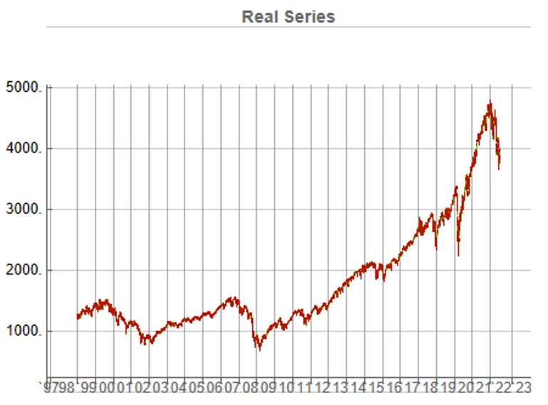
In this demonstration I am using daily O/H/L/C prices for the S&P 500 index for the period from Jan 1999 to July 2022, comprising four price series over 5,297 daily periods.
Synthetic Price Series
Generating ten synthetic series using the algorithm takes around 2 seconds with parallelization. I chose to generate series of the same length as the original, although I could just as easily have produced shorter, or longer sequences.
The first task is to confirm that the synthetic data are internally consistent, and indeed is guaranteed to be so because of the way the algorithm is designed. For example, here are the first few daily bars from the first synthetic series:

This means, of course, that we can immediately plot the synthetic series in a candlestick chart, just as we did with the real data series, above.
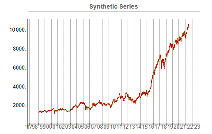
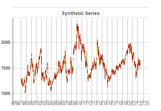
While the real and synthetic series are clearly different, the pattern of peaks and troughs somehow looks recognizably familiar. So, too, is the upward drift in the series, which is this case carries the synthetic S&P 500 Index to a high above 10,000 in 2022. Obviously this is a much more bullish scenario that we have seen in reality. But in fact this is just one example taken from the more “optimistic” end of the spectrum of possibilities. An illustration from the opposite end of the spectrum is shown in the chart below, in which the Index moves sideways over the entire 23 year span, with several very large drawdowns of -20% or more:
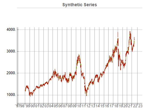
A more typical scenario might look something like our third chart, below. Here, too, we see several very large drawdowns, especially in the period from 2010-2011, but there is also a general upward drift in the process that enables the Index to reach levels comparable to those achieved by the real series:
Price Correlations
Reflecting these very different price path evolutions, we observe large variation in the correlations between the real and synthetic price series. For example:


As these tables indicate, the algorithm is capable of producing replica series that either mimic the original, real price series very closely, or which show completely different behavior, as in the second example.
Dimensionality Reduction
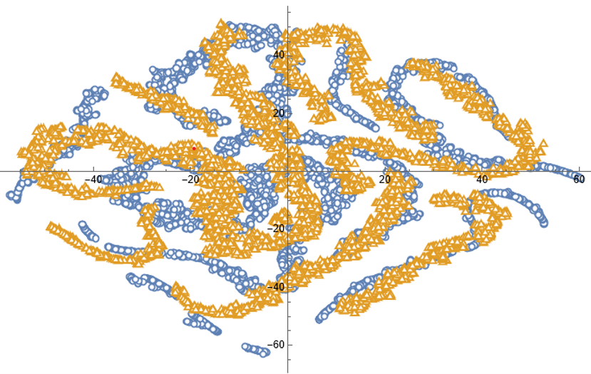
For completeness, as have previous researchers, we apply t-SNE dimensionality reduction and plot the two-factor weightings for both real (yellow) and synthetic data (blue). We observe that while there is considerable overlap in reduced dimensional space, it is not as pronounced as for the synthetic data produced by TimeGAN, for instance. However, as previously explained, we are less concerned by this than we are about the tests previously described, which in our view provide a more appropriate analysis benchmark, so far as market data is concerned. Furthermore, for the reasons previously given, we want synthetic market data that in some cases tracks well beyond the range seen in historical price series.
Returns Distributions
Moving on, we next consider the characteristics of the returns in the synthetic series in comparison to the real data series, where returns are measured as the differences in the Log-Close prices, in the usual way.
Histograms of the returns for the most “optimistic” and “pessimistic” scenarios charted previously are shown below:
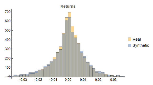
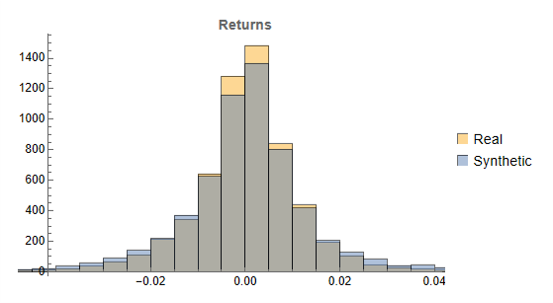
In both cases the distribution of returns in the synthetic series closely matches that of the real returns process and are clearly non-Gaussian, with an over-weighting in the distribution tails. A more detailed look at the distribution characteristics for the first four synthetic series indicates that there is a very good match to the real returns process in each case (the results for other series are very similar):
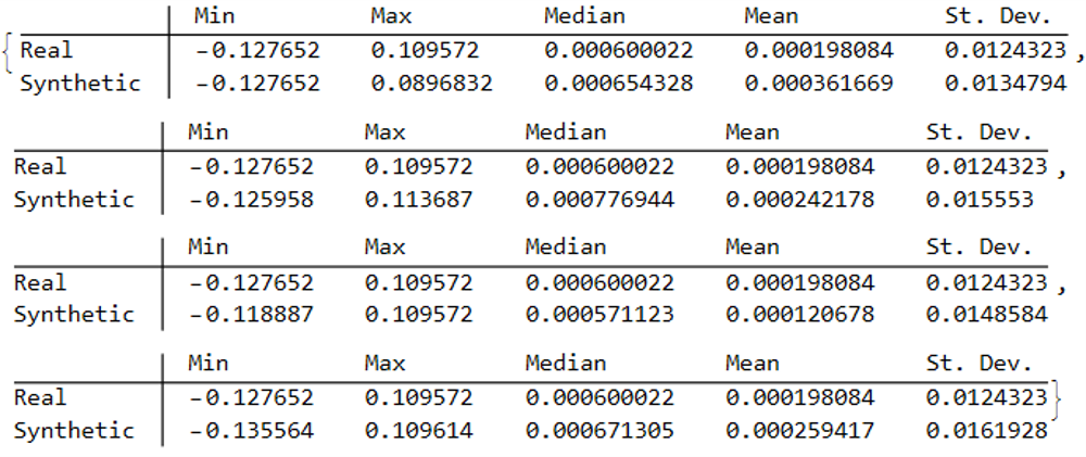
We observe that the minimum and maximum returns of the synthetic series sometimes exceed those of the real series, which can be a useful characteristic for risk management applications. The median and mean of the real and synthetic series are broadly similar, sometimes higher, in other cases lower. Only for the standard deviation of returns do we observe a systematic pattern, in which returns volatility in the synthetic series is consistently higher than in the real series.
This feature, I would argue, is both appropriate and useful. Standard deviations should generally be higher, because there is indeed greater uncertainty about the prices and returns in artificially generated synthetic data, compared to the real series. Moreover, this characteristic is useful, because it will impose a greater stress-test burden on risk management systems compared to simply drawing from the distribution of real returns using Monte Carlo simulation. Put simply, there will be a greater number of more extreme tail events in scenarios using synthetic data, and this will cause risk control parameters to be set more conservatively than they otherwise might. This same characteristic – the greater variation in prices and returns – will also pose a tougher challenge for AI systems that attempt to create trading strategies using genetic programming, meaning that any such strategies are more likely to perform robustly in a live trading environment. I will be returning to this issue in a follow-up post.
Returns Process Characteristics
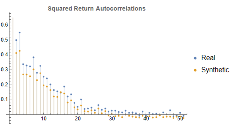
In the following plot we take a look at the autocorrelations in the returns process for a typical synthetic series. These compare closely with the autocorrelations in the real returns series up to 50 lags, which means that any long memory effects are likely to be conserved.
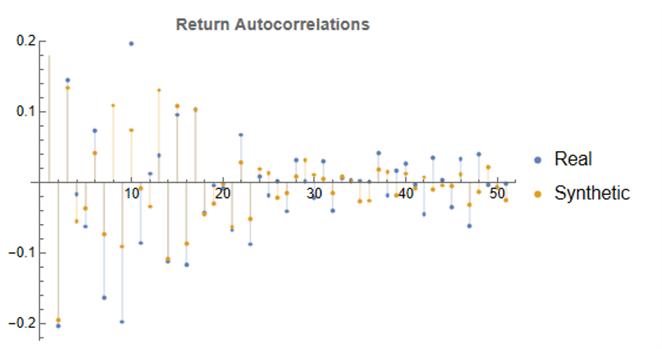
Finally, when we come to consider the autocorrelations in the square of the returns, we observe slowly decaying coefficients over long lags – evidence of so-called GARCH effects – for both real and synthetic series:
Summary
Overall, we observe that the algorithm is capable of generating consistent stock price series that correlate highly with the real price series. It is also capable of generating price series that have low, or even negative, correlation, a feature that may have important applications in the context of risk management. The distribution of returns in the synthetic series closely match those of the real returns process, and moreover retain important features such as long memory and GARCH effects.
Objections to the Use of Synthetic Data
Criticism of synthetic market data (including from myself) has hitherto focused on the inadequacy of such data in terms of representing important characteristics of real data series. Now that such technical issues have been addressed, I will try to anticipate some of the additional concerns that are likely to surface, going forward.
- The Synthetic Data is “Unrealistic”
What is meant here is that there is no plausible set of real, economic factors that would be likely to combine in a way to produce the pattern of prices shown in some of the synthetic data series. The idea that, as observed in one of the artificial scenarios above, the Fed would stand idly by while the market plunged by 50% to 60%, seems highly implausible. Equally unlikely is a scenario in which the market moves sideways for an extended period of a decade, or longer.
To a limited extent, I would agree with this. However, just because such scenarios are currently unlikely doesn’t mean they can never happen. For instance, take a look at the performance of the S&P 500 Index over the period from 1966 through 1979:
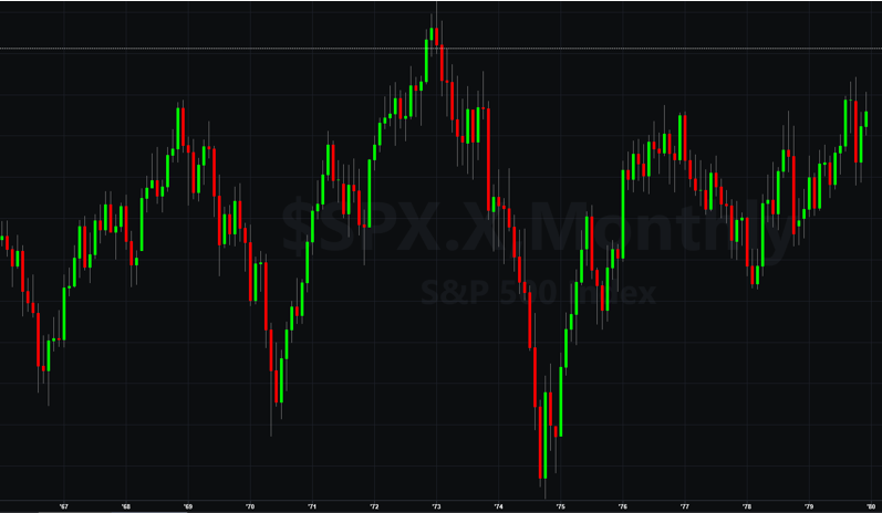
The market index barely made any progress throughout the entire 13-year period, which was characterized by a vicious bout of stagflation. Note, too, the precipitous drop in the index following the oil shock in 1973.
So to say that such scenarios – however implausible they may appear to be – can never happen is simply mistaken.
Finally, let’s not forget that, while the focus of this article is on the US market index, there are many economies, such as Mexico, Brazil or Argentina, for which such adverse developments are much more credible than they might currently be for the United States. We may wish to produce synthetic data for the markets in such economies for modelling purposes, in which case we will want to generate synthetic data capturing the full range of possible market outcomes, including some of the worst-case scenarios.
2. Extreme Scenarios Occur Too Frequently in Synthetic Data
Actually this is not the case – the generator tends to produce extreme scenarios with a frequency that is plausible, given the history and characteristics of the underlying, real price process. But there can be good reasons for wanting to control the frequency of such scenarios.
For instance, an investment manager may be looking to develop a “long-only” investment portfolio because, given his investment remit, that is the only type of investment strategy permitted. He would likely want to limit his focus to the more benign market outcomes for two reasons: (i) his investment thesis is that the market is likely to perform well, going forward (or else how does he pitch his strategy to investors?) and (ii) while he accepts that he may be wrong, it is not his job to hedge a possible market downturn – the responsibility for dealing with an adverse outcome falls to his risk manager, or to the investor.
Conversely, a risk manager is much more likely to be interested in adverse scenarios and, if anything, is likely to want to see such outcomes over-represented in a sample of synthetic data.
The point is, there is no “correct” answer: one has to decide which types of scenarios best suit the application one has in mind and sample the data accordingly. This can be done in a variety of ways such as setting a minimum required correlation between the synthetic and real price series, or designing a system of stratified sampling in which the desired outcomes are sampled according to a stipulated frequency distribution.
3. Synthetic Data Does Not Prevent Data Snooping and Curve Fitting
A critic might argue that, in fact, the real market data is “unseen” only in a theoretical sense, since its essential attributes have been baked into the synthetic series produced by the generator. This applies to an even greater extent if the synthetic series are sampled in some way, as described above.
I think this is a fair point. To take an extreme scenario, one could choose to select only synthetic series for which the correlation with the real data is 99.9%, or higher. Clearly this runs counter to the spirit of what one is trying to achieve with synthetic data and one might just as well use real data for modelling purposes. In practice, of course, even where a sampling methodology is applied, it is unlikely to be as crudely biased as in this example.
But, in any case, what is the alternative? The only option I can see is one in which a pure mathematical model is used to produce synthetic data, without any reference to the underlying real series. But, in that case, how would one assess the validity of the model assumptions, or how representative the synthetic series it produces might be?
There is no alternative but to have recourse to the real data at some point in the modelling process. In this procedure, however, the impact of snooping bias or curve fitting, even though it can never be totally extinguished, is very much diminished and it plays a less central role in model development.
Conclusion
It is now possible to produce synthetic data series that have all of the hallmark characteristics of real price data. This permits the analyst to investigate market models without direct recourse to the real price series, thereby minimizing data snooping and curve fitting bias. Models developed using synthetic data describing many different price path evolutions are more likely to prove robust across a wider range of plausible market scenarios in the real world.
In the next, follow-up post I will illustrate the application of synthetic data to the development of a robust investment strategy.
Volatility Forecasting in Emerging Markets
The great majority of empirical studies have focused on asset markets in the US and other developed economies. The purpose of this research is to determine to what extent the findings of other researchers in relation to the characteristics of asset volatility in developed economies applies also to emerging markets. The important characteristics observed in asset volatility that we wish to identify and examine in emerging markets include clustering, (the tendency for periodic regimes of high or low volatility) long memory, asymmetry, and correlation with the underlying returns process. The extent to which such behaviors are present in emerging markets will serve to confirm or refute the conjecture that they are universal and not just the product of some factors specific to the intensely scrutinized, and widely traded developed markets.
The ten emerging markets we consider comprise equity markets in Australia, Hong Kong, Indonesia, Malaysia, New Zealand, Philippines, Singapore, South Korea, Sri Lanka and Taiwan focusing on the major market indices for those markets. After analyzing the characteristics of index volatility for these indices, the research goes on to develop single- and two-factor REGARCH models in the form by Alizadeh, Brandt and Diebold (2002).
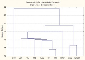
Cluster Analysis of Volatility
Processes for Ten Emerging Market Indices
The research confirms the presence of a number of typical characteristics of volatility processes for emerging markets that have previously been identified in empirical research conducted in developed markets. These characteristics include volatility clustering, long memory, and asymmetry. There appears to be strong evidence of a region-wide regime shift in volatility processes during the Asian crises in 1997, and a less prevalent regime shift in September 2001. We find evidence from multivariate analysis that the sample separates into two distinct groups: a lower volatility group comprising the Australian and New Zealand indices and a higher volatility group comprising the majority of the other indices.
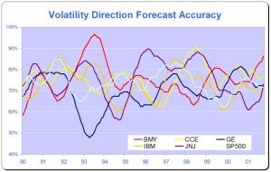
Models developed within the single- and two-factor REGARCH framework of Alizadeh, Brandt and Diebold (2002) provide a good fit for many of the volatility series and in many cases have performance characteristics that compare favorably with other classes of models with high R-squares, low MAPE and direction prediction accuracy of 70% or more. On the debit side, many of the models demonstrate considerable variation in explanatory power over time, often associated with regime shifts or major market events, and this is typically accompanied by some model parameter drift and/or instability.
Single equation ARFIMA-GARCH models appear to be a robust and reliable framework for modeling asset volatility processes, as they are capable of capturing both the short- and long-memory effects in the volatility processes, as well as GARCH effects in the kurtosis process. The available procedures for estimating the degree of fractional integration in the volatility processes produce estimates that appear to vary widely for processes which include both short- and long- memory effects, but the overall conclusion is that long memory effects are at least as important as they are for volatility processes in developed markets. Simple extensions to the single-equation models, which include regressor lags of related volatility series, add significant explanatory power to the models and suggest the existence of Granger-causality relationships between processes.
Extending the modeling procedures into the realm of models which incorporate systems of equations provides evidence of two-way Granger causality between certain of the volatility processes and suggests that are fractionally cointegrated, a finding shared with parallel studies of volatility processes in developed markets.
Download paper here.
Long Memory and Regime Shifts in Asset Volatility
This post covers quite a wide range of concepts in volatility modeling relating to long memory and regime shifts and is based on an article that was published in Wilmott magazine and republished in The Best of Wilmott Vol 1 in 2005. A copy of the article can be downloaded here.
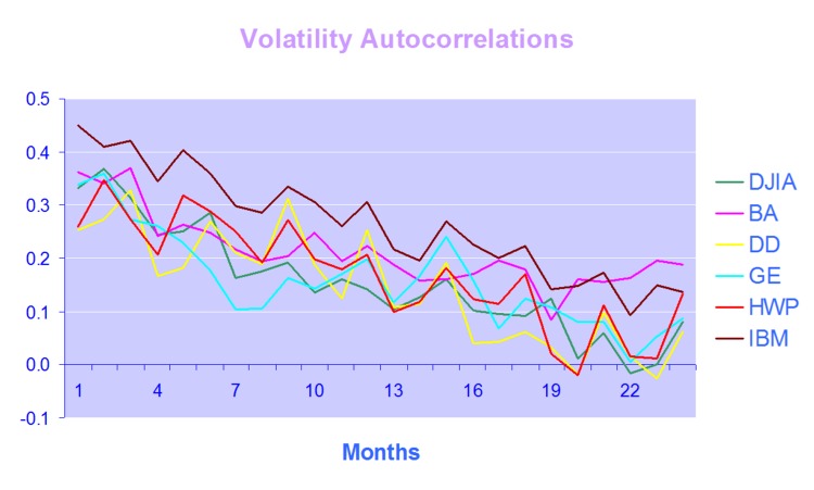
One of the defining characteristics of volatility processes in general (not just financial assets) is the tendency for the serial autocorrelations to decline very slowly. This effect is illustrated quite clearly in the chart below, which maps the autocorrelations in the volatility processes of several financial assets.
Thus we can say that events in the volatility process for IBM, for instance, continue to exert influence on the process almost two years later.
This feature in one that is typical of a black noise process – not some kind of rap music variant, but rather:
“a process with a 1/fβ spectrum, where β > 2 (Manfred Schroeder, “Fractals, chaos, power laws“). Used in modeling various environmental processes. Is said to be a characteristic of “natural and unnatural catastrophes like floods, droughts, bear markets, and various outrageous outages, such as those of electrical power.” Further, “because of their black spectra, such disasters often come in clusters.”” [Wikipedia].
Because of these autocorrelations, black noise processes tend to reinforce or trend, and hence (to some degree) may be forecastable. This contrasts with a white noise process, such as an asset return process, which has a uniform power spectrum, insignificant serial autocorrelations and no discernable trending behavior:
An econometrician might describe this situation by saying that a black noise process is fractionally integrated order d, where d = H/2, H being the Hurst Exponent. A way to appreciate the difference in the behavior of a black noise process vs. a white process is by comparing two fractionally integrated random walks generated using the same set of quasi random numbers by Feder’s (1988) algorithm (see p 32 of the presentation on Modeling Asset Volatility).
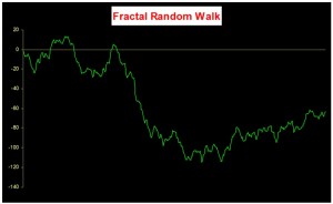
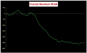
As you can see. both random walks follow a similar pattern, but the black noise random walk is much smoother, and the downward trend is more clearly discernible. You can play around with the Feder algorithm, which is coded in the accompanying Excel Workbook on Volatility and Nonlinear Dynamics . Changing the Hurst Exponent parameter H in the worksheet will rerun the algorithm and illustrate a fractal random walk for a black noise (H > 0.5), white noise (H=0.5) and mean-reverting, pink noise (H<0.5) process.
One way of modeling the kind of behavior demonstrated by volatility process is by using long memory models such as ARFIMA and FIGARCH (see pp 47-62 of the Modeling Asset Volatility presentation for a discussion and comparison of various long memory models). The article reviews research into long memory behavior and various techniques for estimating long memory models and the coefficient of fractional integration d for a process.
But long memory is not the only possible cause of long term serial correlation. The same effect can result from structural breaks in the process, which can produce spurious autocorrelations. The article goes on to review some of the statistical procedures that have been developed to detect regime shifts, due to Bai (1997), Bai and Perron (1998) and the Iterative Cumulative Sums of Squares methodology due to Aggarwal, Inclan and Leal (1999). The article illustrates how the ICSS technique accurately identifies two changes of regimes in a synthetic GBM process.
In general, I have found the ICSS test to be a simple and highly informative means of gaining insight about a process representing an individual asset, or indeed an entire market. For example, ICSS detects regime shifts in the process for IBM around 1984 (the time of the introduction of the IBM PC), the automotive industry in the early 1980’s (Chrysler bailout), the banking sector in the late 1980’s (Latin American debt crisis), Asian sector indices in Q3 1997, the S&P 500 index in April 2000 and just about every market imaginable during the 2008 credit crisis. By splitting a series into pre- and post-regime shift sub-series and examining each segment for long memory effects, one can determine the cause of autocorrelations in the process. In some cases, Asian equity indices being one example, long memory effects disappear from the series, indicating that spurious autocorrelations were induced by a major regime shift during the 1997 Asian crisis. In most cases, however, long memory effects persist.
Excel Workbook on Volatility and Nonlinear Dynamics
There are several other topics from chaos theory and nonlinear dynamics covered in the workbook, including:
- Generation of the Sierpinski triangle
- Estimation of the Hurst Exponent in various series (Industrial Production, DJIA, S&P500)
- Logistic and Henon attractors
- Estimation of the fractal dimension and correlation integral for the S&P500 index
More on these issues in due course.
Modeling Asset Volatility
I am planning a series of posts on the subject of asset volatility and option pricing and thought I would begin with a survey of some of the central ideas. The attached presentation on Modeling Asset Volatility sets out the foundation for a number of key concepts and the basis for the research to follow.
Perhaps the most important feature of volatility is that it is stochastic rather than constant, as envisioned in the Black Scholes framework. The presentation addresses this issue by identifying some of the chief stylized facts about volatility processes and how they can be modelled. Certain characteristics of volatility are well known to most analysts, such as, for instance, its tendency to “cluster” in periods of higher and lower volatility. However, there are many other typical features that are less often rehearsed and these too are examined in the presentation.
Long Memory
For example, while it is true that GARCH models do a fine job of modeling the clustering effect they typically fail to capture one of the most important features of volatility processes – long term serial autocorrelation. In the typical GARCH model autocorrelations die away approximately exponentially, and historical events are seen to have little influence on the behaviour of the process very far into the future. In volatility processes that is typically not the case, however: autocorrelations die away very slowly and historical events may continue to affect the process many weeks, months or even years ahead.
There are two immediate and very important consequences of this feature. The first is that volatility processes will tend to trend over long periods – a characteristic of Black Noise or Fractionally Integrated processes, compared to the White Noise behavior that typically characterizes asset return processes. Secondly, and again in contrast with asset return processes, volatility processes are inherently predictable, being conditioned to a significant degree on past behavior. The presentation considers the fractional integration frameworks as a basis for modeling and forecasting volatility.
Mean Reversion vs. Momentum
A puzzling feature of much of the literature on volatility is that it tends to stress the mean-reverting behavior of volatility processes. This appears to contradict the finding that volatility behaves as a reinforcing process, whose long-term serial autocorrelations create a tendency to trend. This leads to one of the most important findings about asset processes in general, and volatility process in particular: i.e. that the assets processes are simultaneously trending and mean-reverting. One way to understand this is to think of volatility, not as a single process, but as the superposition of two processes: a long term process in the mean, which tends to reinforce and trend, around which there operates a second, transient process that has a tendency to produce short term spikes in volatility that decay very quickly. In other words, a transient, mean reverting processes inter-linked with a momentum process in the mean. The presentation discusses two-factor modeling concepts along these lines, and about which I will have more to say later.
Cointegration
One of the most striking developments in econometrics over the last thirty years, cointegration is now a principal weapon of choice routinely used by quantitative analysts to address research issues ranging from statistical arbitrage to portfolio construction and asset allocation. Back in the late 1990’s I and a handful of other researchers realized that volatility processes exhibited very powerful cointegration tendencies that could be harnessed to create long-short volatility strategies, mirroring the approach much beloved by equity hedge fund managers. In fact, this modeling technique provided the basis for the Caissa Capital volatility fund, which I founded in 2002. The presentation examines characteristics of multivariate volatility processes and some of the ideas that have been proposed to model them, such as FIGARCH (fractionally-integrated GARCH).
Dispersion Dynamics
Finally, one topic that is not considered in the presentation, but on which I have spent much research effort in recent years, is the behavior of cross-sectional volatility processes, which I like to term dispersion. It turns out that, like its univariate cousin, dispersion displays certain characteristics that in principle make it highly forecastable. Given an appropriate model of dispersion dynamics, the question then becomes how to monetize efficiently the insight that such a model offers. Again, I will have much more to say on this subject, in future.
Forecasting Volatility in the S&P500 Index
Several people have asked me for copies of this research article, which develops a new theoretical framework, the ARFIMA-GARCH model as a basis for forecasting volatility in the S&P 500 Index. I am in the process of updating the research, but in the meantime a copy of the original paper is available here
In this analysis we are concerned with the issue of whether market forecasts of volatility, as expressed in the Black-Scholes implied volatilities of at-the-money European options on the S&P500 Index, are superior to those produced by a new forecasting model in the GARCH framework which incorporates long-memory effects. The ARFIMA-GARCH model, which uses high frequency data comprising 5-minute returns, makes volatility the subject process of interest, to which innovations are introduced via a volatility-of-volatility (kurtosis) process. Despite performing robustly in- and out-of-sample, an encompassing regression indicates that the model is unable to add to the information already contained in market forecasts. However, unlike model forecasts, implied volatility forecasts show evidence of a consistent and substantial bias. Furthermore, the model is able to correctly predict the direction of volatility approximately 62% of the time whereas market forecasts have very poor direction prediction ability. This suggests that either option markets may be inefficient, or that the option pricing model is mis-specified. To examine this hypothesis, an empirical test is carried out in which at-the-money straddles are bought or sold (and delta-hedged) depending on whether the model forecasts exceed or fall below implied volatility forecasts. This simple strategy generates an annual compound return of 18.64% over a four year out-of-sample period, during which the annual return on the S&P index itself was -7.24%. Our findings suggest that, over the period of analysis, investors required an additional risk premium of 88 basis points of incremental return for each unit of volatility risk.
Modeling Asset Processes
Introduction
Over the last twenty five years significant advances have been made in the theory of asset processes and there now exist a variety of mathematical models, many of them computationally tractable, that provide a reasonable representation of their defining characteristics.
While the Geometric Brownian Motion model remains a staple of stochastic calculus theory, it is no longer the only game in town. Other models, many more sophisticated, have been developed to address the shortcomings in the original. There now exist models that provide a good explanation of some of the key characteristics of asset processes that lie beyond the scope of models couched in a simple Gaussian framework. Features such as mean reversion, long memory, stochastic volatility, jumps and heavy tails are now readily handled by these more advanced tools.
In this post I review a critical selection of asset process models that belong in every financial engineer’s toolbox, point out their key features and limitations and give examples of some of their applications.
Falling Water
The current 15-year drought in the South West is the most severe since recordkeeping for the Colorado River began in 1906. Lake Mead, which supplies much of the water to Colorado Basin communities, is now more than half empty.
A 120 foot high band of rock, bleached white by the water, and known as the “bathtub ring” encircles the lake, a stark reminder of the water crisis that has enveloped the surrounding region. The Colorado River takes a 1,400 mile journey from the Rockies to Mexico, irrigating over 5 million acres of farmland in the Basin states of Wyoming, Utah, Colorado, New Mexico, Nevada, Arizona, and California.
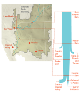
The Colorado River Compact signed in 1922 enshrined the States’ water rights in law and Mexico was added to the roster in 1994, taking the total allocation to over 16.5 million acre-feet per year. But the average freshwater input to the lake over the century from 1906 to 2005 reached only 15 million acre-feet. The river can’t come close to meeting current demand and the problem is only likely to get worse. A 2009 study found that rainfall in the Colorado Basin could fall as much as 15% over the next 50 years and the shortfall in deliveries could reach 60% to 90% of the time.
Impact on Las Vegas
With an average of only 4 inches of rain a year, and a daily high temperatures of 103 o F during the summer, Las Vegas is perhaps the most hard pressed to meet the demand of its 2 million residents and 40 million visitors annually. 
Despite its conspicuous consumption, from the tumbling fountains of the Bellagio to the Venetian’s canals, since 2002, Las Vegas has been obliged to cut its water use by a third, from 314 gallons per capita a day to 212. The region recycles around half of its wastewater which is piped back into Lake Mead, after cleaning and treatment. Residents are allowed to water their gardens no more than one day a week in peak season, and there are stiff fines for noncompliance.
The Third Straw
Historically, two intake pipes carried water from Lake Mead to Las Vegas, about 25 miles to the west. In 2012, realizing that the highest of these, at 1050 feet, would soon be sucking air, the Southern Nevada Water Authority began construction of a new pipeline. Known as the Third Straw, Intake No. 3 reaches 200 feet deeper into the lake—to keep water flowing for as long as there’s water to pump. The new pipeline, which commenced operations in 2015, doesn’t draw more water from the lake than before, or make the surface level drop any faster. But it will keep taps flowing in Las Vegas homes and casinos even if drought-stricken Lake Mead drops to its lowest levels.

Modeling Water Levels in Lake Mead
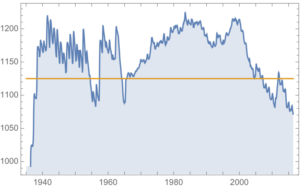
The monthly reported water levels in Lake Mead from Feb 1935 to June 2016 are shown in the chart below. The reference line is the drought level, historically defined as 1,125 feet.
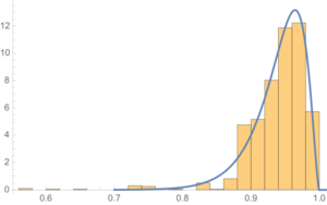
One statistical technique widely applied in hydrology involves fitting a Kumaraswamy distribution to the relative water level. According to the Arizona Game and Fish Department, the maximum lake level is 1229 feet. We model the water level relative to the maximum level, as follows.
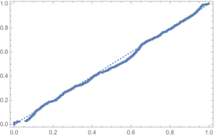
The fit of the distribution appears quite good, even in the tails:
ProbabilityPlot[relativeLevels, edist]
Since water levels have been below the drought level for some time, let’s instead consider the “emergency” level, 1,075 feet. According to this model, there is just over a 6% chance of Lake Mead hitting the emergency level and, consequently, a high probability of breaching the emergency threshold some time over before the end of 2017.
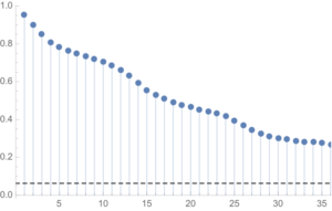
One problem with this approach is that it assumes that each observation is drawn independently from a random variable with the estimated distribution. In reality, there are high levels of autocorrelation in the series, as might be expected: lower levels last month typically increase the likelihood of lower levels this month. The chart of the autocorrelation coefficients makes this pattern clear, with statistically significant coefficients at lags of up to 36 months.
ts[“ACFPlot”]
An alternative methodology that enables us to take account of the autocorrelation in the process is time series analysis. We proceed to fit an autoregressive moving average (ARMA) model as follows:
tsm = TimeSeriesModelFit[ts, “ARMA”]
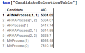
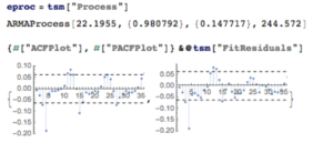
The best fitting model in an ARMA(1,1) model, according to the AIC criterion:
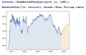
Applying the fitted ARMA model, we forecast the water level in Lake Mead over the next ten years as shown in the chart below. Given the mean-reverting moving average component of the model, it is not surprising to see the model forecasting a return to normal levels.
There is some evidence of lack of fit in the ARMA model, as shown in the autocorrelations of the model residuals:
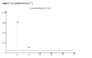
A formal test reveals that residual autocorrelations at lags 4 and higher are jointly statistically significant:
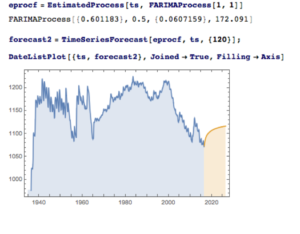
The slowly decaying pattern of autocorrelations in the water level series suggests a possible “long memory” effect, which can be better modelled as a fractionally integrated process. The forecasts from such a model, like the ARMA model forecasts, display a tendency to revert to a long term mean; but the reversion process is dampened by the reinforcing, long-memory effect captured in the FARIMA model.
The Prospects for the Next Decade
Taking the view that the water level in Lake Mead forms a stationary statistical process, the likelihood is that water levels will rise to 1,125 feet or more over the next ten years, easing the current water shortage in the region.
On the other hand, there are good reasons to believe that there are exogenous (deterministic) factors in play, specifically the over-consumption of water at a rate greater than the replenishment rate from average rainfall levels. Added to this, plausible studies suggest that average rainfall in the Colorado Basin is expected to decline over the next fifty years. Under this scenario, the water level in Lake Mead will likely continue to deteriorate, unless more stringent measures are introduced to regulate consumption.
Economic Impact
The drought in the South West affects far more than just the water levels in Lake Mead, of course. One study found that California’s agriculture sector alone had lost $2.2Bn and some 17,00 season and part time jobs in 2014, due to drought. Agriculture uses more than 80% of the State’s water, according to Fortune magazine, which goes on to identify the key industries most affected, including agriculture, food processing, semiconductors, energy, utilities and tourism.

In the energy sector, for example, the loss of hydroelectric power cost CA around $1.4Bn in 2014, according to non-profit research group Pacific Institute. Although Intel pulled its last fabrication plant from California in 2009, semiconductor manufacturing is still a going concern in the state. Maxim Integrated, TowerJazz, and TSI Semiconductors all still have fabrication plants in the state. And they need a lot of water. A single semiconductor fabrication plant can use as much water as a small city. That means the current plants could represent three cities worth of consumption.
The drought is also bad news for water utilities, of course. The need to conserve water raises the priority on repair and maintenance, and that means higher costs and lower profit. Complicating the problem, California lacks any kind of management system for its water supply and can’t measure the inflows and outflows to ground water levels at any particular time.
The Bureau of Reclamation has studied more than two dozen options for conserving and increasing water supply, including importation, desalination and reuse. While some were disregarded for being too costly or difficult, the bureau found that the remaining options, if instituted, could yield 3.7 million acre feet per year in savings and new supplies, increasing to 7 million acre feet per year by 2060. Agriculture is the biggest user by far and has to be part of any solution. In the near term, the agriculture industry could reduce its use by 10 to 15 percent without changing the types of crops it grows by using new technology, such as using drip irrigation instead of flood irrigation and monitoring soil moisture to prevent overwatering, the Pacific Institute found.
Conclusion
We can anticipate that a series of short term fixes, like the “Third Straw”, will be employed to kick the can down the road as far as possible, but research now appears almost unanimous in finding that drought is having a deleterious, long term affect on the economics of the South Western states. Agriculture is likely to have to bear the brunt of the impact, but so too will adverse consequences be felt in industries as disparate as food processing, semiconductors and utilities. California, with the largest agricultural industry, by far, is likely to be hardest hit. The Las Vegas region may be far less vulnerable, having already taken aggressive steps to conserve and reuse water supply and charge economic rents for water usage.
Modeling Water Levels in Lake Mead
The monthly reported water levels in Lake Mead from Feb 1935 to June 2016 are shown in the chart below. The reference line is the drought level, historically defined as 1,125 feet.
One statistical technique widely applied in hydrology involves fitting a Kumaraswamy distribution to the relative water level. According to the Arizona Game and Fish Department, the maximum lake level is 1229 feet. We model the water level relative to the maximum level, as follows.
The fit of the distribution appears quite good, even in the tails:
ProbabilityPlot[relativeLevels, edist]
Since water levels have been below the drought level for some time, let’s instead consider the “emergency” level, 1,075 feet. According to this model, there is just over a 6% chance of Lake Mead hitting the emergency level and, consequently, a high probability of breaching the emergency threshold some time over before the end of 2017.
One problem with this approach is that it assumes that each observation is drawn independently from a random variable with the estimated distribution. In reality, there are high levels of autocorrelation in the series, as might be expected: lower levels last month typically increase the likelihood of lower levels this month. The chart of the autocorrelation coefficients makes this pattern clear, with statistically significant coefficients at lags of up to 36 months.
ts[“ACFPlot”]
An alternative methodology that enables us to take account of the autocorrelation in the process is time series analysis. We proceed to fit an autoregressive moving average (ARMA) model as follows:
tsm = TimeSeriesModelFit[ts, “ARMA”]
The best fitting model in an ARMA(1,1) model, according to the AIC criterion:
Applying the fitted ARMA model, we forecast the water level in Lake Mead over the next ten years as shown in the chart below. Given the mean-reverting moving average component of the model, it is not surprising to see the model forecasting a return to normal levels.
There is some evidence of lack of fit in the ARMA model, as shown in the autocorrelations of the model residuals:
A formal test reveals that residual autocorrelations at lags 4 and higher are jointly statistically significant:
The slowly decaying pattern of autocorrelations in the water level series suggests a possible “long memory” effect, which can be better modelled as a fractionally integrated process. The forecasts from such a model, like the ARMA model forecasts, display a tendency to revert to a long term mean; but the reversion process is dampened by the reinforcing, long-memory effect captured in the FARIMA model.
The Prospects for the Next Decade
Taking the view that the water level in Lake Mead forms a stationary statistical process, the likelihood is that water levels will rise to 1,125 feet or more over the next ten years, easing the current water shortage in the region.
On the other hand, there are good reasons to believe that there are exogenous (deterministic) factors in play, specifically the over-consumption of water at a rate greater than the replenishment rate from average rainfall levels. Added to this, plausible studies suggest that average rainfall in the Colorado Basin is expected to decline over the next fifty years. Under this scenario, the water level in Lake Mead will likely continue to deteriorate, unless more stringent measures are introduced to regulate consumption.
Economic Impact
The drought in the South West affects far more than just the water levels in Lake Mead, of course. One study found that California’s agriculture sector alone had lost $2.2Bn and some 17,00 season and part time jobs in 2014, due to drought. Agriculture uses more than 80% of the State’s water, according to Fortune magazine, which goes on to identify the key industries most affected, including agriculture, food processing, semiconductors, energy, utilities and tourism.
In the energy sector, for example, the loss of hydroelectric power cost CA around $1.4Bn in 2014, according to non-profit research group Pacific Institute.
Although Intel pulled its last fabrication plant from California in 2009, semiconductor manufacturing is still a going concern in the state. Maxim Integrated, TowerJazz, and TSI Semiconductors all still have fabrication plants in the state. And they need a lot of water. A single semiconductor fabrication plant can use as much water as a small city. That means the current plants could represent three cities worth of consumption.
The drought is also bad news for water utilities, of course. The need to conserve water raises the priority on repair and maintenance, and that means higher costs and lower profit. Complicating the problem, California lacks any kind of management system for its water supply and can’t measure the inflows and outflows to ground water levels at any particular time.
The Bureau of Reclamation has studied more than two dozen options for conserving and increasing water supply, including importation, desalination and reuse. While some were disregarded for being too costly or difficult, the bureau found that the remaining options, if instituted, could yield 3.7 million acre feet per year in savings and new supplies, increasing to 7 million acre feet per year by 2060. Agriculture is the biggest user by far and has to be part of any solution. In the near term, the agriculture industry could reduce its use by 10 to 15 percent without changing the types of crops it grows by using new technology, such as using drip irrigation instead of flood irrigation and monitoring soil moisture to prevent overwatering, the Pacific Institute found.
Conclusion
We can anticipate that a series of short term fixes, like the “Third Straw”, will be employed to kick the can down the road as far as possible, but research now appears almost unanimous in finding that drought is having a deleterious, long term affect on the economics of the South Western states. Agriculture is likely to have to bear the brunt of the impact, but so too will adverse consequences be felt in industries as disparate as food processing, semiconductors and utilities. California, with the largest agricultural industry, by far, is likely to be hardest hit. The Las Vegas region may be far less vulnerable, having already taken aggressive steps to conserve and reuse water supply and charge economic rents for water usage.

