
Introduction
If you’ve been trading anything other than cash over the past eighteen months, you’ve noticed something peculiar: periods of calm tend to persist, but so do periods of chaos. A quiet Tuesday in January rarely suddenly explodes into volatility on Wednesday—market turbulence comes in clusters. This isn’t market inefficiency; it’s a fundamental stylized fact of financial markets, one that most quant models fail to properly account for.
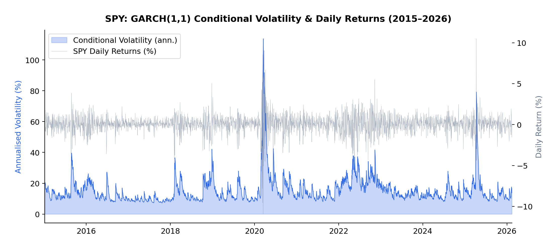
The current volatility regime we’re navigating in early 2026 provides a perfect case study. Following the Federal Reserve’s policy pivot late in 2025, equity markets experienced a sharp correction, with the VIX spiking from around 15 to above 30 in a matter of weeks. But here’s what interests me as a researcher: that elevated volatility didn’t dissipate overnight. It lingered, exhibiting the characteristic “slow decay” that the GARCH framework was designed to capture.
In this article, I present an empirical analysis of volatility dynamics across five major asset classes—the S&P 500 (SPY), US Treasuries (TLT), Gold (GLD), Oil (USO), and Bitcoin (BTC-USD)—over the ten-year period from January 2015 to February 2026. Using both GARCH(1,1) and EGARCH(1,1,1) models, I characterize volatility persistence and leverage effects, revealing striking differences across asset classes that have direct implications for risk management and trading strategy design.
This extends my earlier work on VIX derivatives and correlation trading, where understanding the time-varying nature of volatility is essential for pricing complex derivatives and managing portfolio risk through volatile regimes.
Understanding Volatility Clustering
Before diving into the results, let’s build some intuition about what GARCH actually captures—and why it matters.
Volatility clustering refers to the empirical observation that large price changes tend to be followed by large price changes, and small changes tend to follow small changes. If the market experiences a turbulent day, don’t expect immediate tranquility the next day. Conversely, a period of quiet trading often continues uninterrupted.
This phenomenon was formally modeled by Robert Engle in his landmark 1982 paper, “Autoregressive Conditional Heteroskedasticity with Estimates of the Variance of United Kingdom Inflation,” which introduced the ARCH (Autoregressive Conditional Heteroskedasticity) model. Engle’s insight was revolutionary: rather than assuming constant variance (homoskedasticity), he modeled variance itself as a time-varying process that depends on past shocks.
Tim Bollerslev extended this work in 1986 with the GARCH (Generalized ARCH) model, which proved more parsimonious and flexible. Then, in 1991, Daniel Nelson introduced the EGARCH (Exponential GARCH) model, which could capture the asymmetric response of volatility to positive versus negative returns—the famous “leverage effect” where negative shocks tend to increase volatility more than positive shocks of equal magnitude.
The Mathematics
The standard GARCH(1,1) model specifies:
where:
- σt2 is the conditional variance at time t
- rt-12 is the squared return from the previous period (the “shock”)
- σt-12 is the previous period’s conditional variance
- α measures how quickly volatility responds to new shocks
- β measures the persistence of volatility shocks
- The sum α + β represents overall volatility persistence
The key parameter here is α + β. If this sum is close to 1 (as it typically is for financial assets), volatility shocks decay slowly—a phenomenon I observed firsthand during the 2025-2026 correction. We can calculate the “half-life” of a volatility shock as:
For example, with α + β = 0.97, a volatility shock takes approximately ln(0.5)/ln(0.97) ≈ 23 days to decay by half.
The EGARCH model modifies this framework to capture asymmetry:
The parameter γ (gamma) captures the leverage effect. A negative γ means that negative returns generate more volatility than positive returns of equal magnitude—which is precisely what we observe in equity markets and, as we’ll see, in Bitcoin.
Methodology
For each asset in the sample, I computed daily log returns as:
The multiplication by 100 converts returns to percentage terms, which improves numerical convergence when estimating the models.
I then fitted two volatility models to each asset’s return series:
- GARCH(1,1): The workhorse model that captures volatility clustering through the autoregressive structure of conditional variance
- EGARCH(1,1,1): The exponential GARCH model that additionally captures leverage effects through the asymmetric term
All models were estimated using Python’s arch package with normally distributed innovations. The sample period spans January 2015 to February 2026, encompassing multiple distinct volatility regimes including:
- The 2015-2016 oil price collapse
- The 2018 Q4 correction
- The COVID-19 volatility spike of March 2020
- The 2022 rate-hike cycle
- The 2025-2026 post-pivot correction
This rich variety of regimes makes the sample ideal for studying volatility dynamics across different market conditions.
Results
GARCH(1,1) Estimates
The GARCH(1,1) model reveals substantial variation in volatility dynamics across asset classes:
| Asset | α (alpha) | β (beta) | Persistence (α+β) | Half-life (days) | AIC |
|---|---|---|---|---|---|
| S&P 500 | 0.1810 | 0.7878 | 0.9688 | ~23 | 7130.4 |
| US Treasuries | 0.0683 | 0.9140 | 0.9823 | ~38 | 7062.7 |
| Gold | 0.0631 | 0.9110 | 0.9741 | ~27 | 7171.9 |
| Oil | 0.1271 | 0.8305 | 0.9576 | ~16 | 11999.4 |
| Bitcoin | 0.1228 | 0.8470 | 0.9699 | ~24 | 20789.6 |
EGARCH(1,1,1) Estimates
The EGARCH model additionally captures leverage effects:
| Asset | α (alpha) | β (beta) | γ (gamma) | Persistence | AIC |
|---|---|---|---|---|---|
| S&P 500 | 0.2398 | 0.9484 | -0.1654 | 1.1882 | 7022.6 |
| US Treasuries | 0.1501 | 0.9806 | 0.0084 | 1.1307 | 7063.5 |
| Gold | 0.1205 | 0.9721 | 0.0452 | 1.0926 | 7146.9 |
| Oil | 0.2171 | 0.9564 | -0.0668 | 1.1735 | 12002.8 |
| Bitcoin | 0.2505 | 0.9377 | -0.0383 | 1.1882 | 20773.9 |
Interpretation
Volatility Persistence
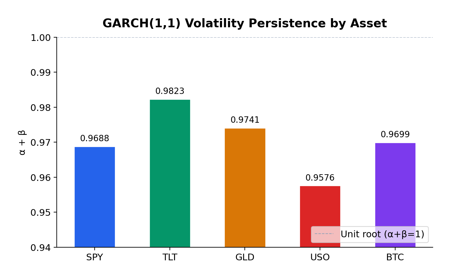
All five assets exhibit high volatility persistence, with α + β ranging from 0.9576 (Oil) to 0.9823 (US Treasuries). These values are remarkably consistent with the classic empirical findings from Engle (1982) and Bollerslev (1986), who first documented this phenomenon in inflation and stock market data respectively.
US Treasuries show the highest persistence (0.9823), meaning volatility shocks in the bond market take longer to decay—approximately 38 days to half-life. This makes intuitive sense: Federal Reserve policy changes, which are the primary drivers of Treasury volatility, tend to have lasting effects that persist through subsequent meetings and economic data releases.
Gold exhibits the second-highest persistence (0.9741), consistent with its role as a long-term store of value. Macroeconomic uncertainties—geopolitical tensions, currency debasement fears, inflation scares—don’t resolve quickly, and neither does the associated volatility.
S&P 500 and Bitcoin show similar persistence (~0.97), with half-lives of approximately 23-24 days. This suggests that equity market volatility shocks, despite their reputation for sudden spikes, actually decay at a moderate pace.
Oil has the lowest persistence (0.9576), which makes sense given the more mean-reverting nature of commodity prices. Oil markets can experience rapid shifts in sentiment based on supply disruptions or demand changes, but these shocks tend to resolve more quickly than in financial assets.
Leverage Effects
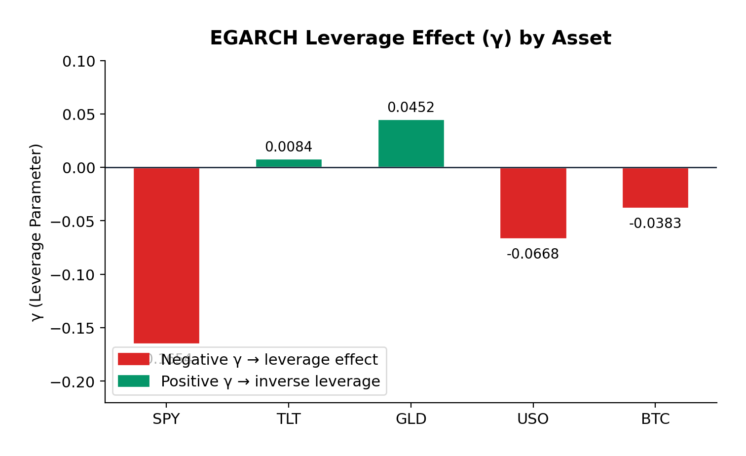
The EGARCH γ parameter reveals asymmetric volatility responses—the leverage effect that Nelson (1991) formalized:
S&P 500 (γ = -0.1654): The strongest negative leverage effect in the sample. A 1% drop in equities increases volatility significantly more than a 1% rise. This is the classic equity pattern: bad news is “stickier” than good news. For options traders, this means that protective puts are more expensive than equivalent out-of-the-money calls during volatile periods—a direct consequence of this asymmetry.
Bitcoin (γ = -0.0383): Moderate negative leverage, weaker than equities but still significant. The cryptocurrency market shows asymmetric reactions to price movements, with downside moves generating more volatility than upside moves. This is somewhat surprising given Bitcoin’s retail-dominated nature, but consistent with the hypothesis that large institutional players are increasingly active in crypto markets.
Oil (γ = -0.0668): Moderate negative leverage, similar to Bitcoin. The energy market’s reaction to geopolitical events (which tend to be negative supply shocks) contributes to this asymmetry.
Gold (γ = +0.0452): Here’s where it gets interesting. Gold exhibits a slight positive gamma—the opposite of the equity pattern. Positive returns slightly increase volatility more than negative returns. This is consistent with gold’s safe-haven role: when risk assets sell off and investors flee to gold, the resulting price spike in gold can be accompanied by increased trading activity and volatility. Conversely, gradual gold price increases during calm markets occur with declining volatility.
US Treasuries (γ = +0.0084): Essentially symmetric. Treasury volatility doesn’t distinguish between positive and negative returns—which makes sense, since Treasuries are priced primarily on interest rate expectations rather than “good” or “bad” news in the equity sense.
Model Fit
The AIC (Akaike Information Criterion) comparison shows that EGARCH provides a materially better fit for the S&P 500 (7022.6 vs 7130.4) and Bitcoin (20773.9 vs 20789.6), where significant leverage effects are present. For Gold and Treasuries, GARCH performs comparably or slightly better, consistent with the absence of significant leverage asymmetry.
Practical Implications for Traders
1. Volatility Forecasting and Position Sizing
The high persistence values across all assets have direct implications for position sizing during volatile regimes. If you’re trading options or managing a portfolio, the GARCH framework tells you that elevated volatility will likely persist for weeks, not days. This suggests:
- Don’t reduce risk too quickly after a volatility spike. The half-life analysis shows that it takes 2-4 weeks for half of a volatility shock to dissipate. Cutting exposure immediately after a correction means you’re selling low vol into the spike.
- Expect re-leveraging opportunities. Once vol peaks and begins decaying, there’s a window of several weeks where volatility is still elevated but declining—potentially favorable for selling vol (e.g., writing covered calls or selling volatility swaps).
2. Options Pricing
The leverage effects have material implications for option pricing:
- Equity options (S&P 500) should price in significant skew—put options are relatively more expensive than calls. If you’re buying protection (e.g., buying SPY puts for portfolio hedge), you’re paying a premium for this asymmetry.
- Bitcoin options show similar but weaker asymmetry. The market is still relatively young, and the vol surface may not fully price in the leverage effect—potentially an edge for sophisticated options traders.
- Gold options exhibit the opposite pattern. Call options may be relatively cheaper than puts, reflecting gold’s tendency to experience vol spikes on rallies (as opposed to selloffs).
3. Portfolio Construction
For multi-asset portfolios, the differing persistence and leverage characteristics suggest tactical allocation shifts:
- During risk-on regimes: Low persistence in oil suggests faster mean reversion—commodity exposure might be appropriate for shorter time horizons.
- During risk-off regimes: High persistence in Treasuries means bond market volatility decays slowly. Duration hedges need to account for this extended volatility window.
- Diversification benefits: The low correlation between equity and Treasury volatility dynamics supports the case for mixed-asset portfolios—but the high persistence in both suggests that when one asset class enters a high-vol regime, it likely persists for weeks.
4. Trading Volatility Directly
For traders who express views on volatility itself (VIX futures, variance swaps, volatility ETFs):
- The persistence framework suggests that VIX spikes should be traded as mean-reverting (which they are), but with the expectation that complete normalization takes 30-60 days.
- The leverage effect in equities means that vol strategies should be positioned for asymmetric payoffs—long vol positions benefit more from downside moves than equivalent upside moves.
Reproducible Example
At the bottom of the post is the complete Python code used to generate these results. The code uses yfinance for data download and the arch package for model estimation. It’s designed to be easily extensible—you can add additional assets, change the date range, or experiment with different GARCH variants (GARCH-M, TGARCH, GJR-GARCH) to capture different aspects of the volatility dynamics.
Conclusion
This analysis confirms that volatility clustering is a universal phenomenon across asset classes, but the specific characteristics vary meaningfully:
- Volatility persistence is universally high (α + β ≈ 0.95–0.98), meaning volatility shocks take weeks to months to decay. This has important implications for position sizing and risk management.
- Leverage effects vary dramatically across asset classes. Equities show strong negative leverage (bad news increases vol more than good news), while gold shows slight positive leverage (opposite pattern), and Treasuries show no meaningful asymmetry.
- The half-life of volatility shocks ranges from approximately 16 days (oil) to 38 days (Treasuries), providing a quantitative guide for expected duration of volatile regimes.
These findings extend naturally to my ongoing work on volatility derivatives and correlation trading. Understanding the persistence and asymmetry of volatility is essential for pricing VIX options, variance swaps, and other vol-sensitive products—as well as for managing the tail risk that inevitably accompanies high-volatility regimes like the one we’re navigating in early 2026.
References
- Engle, R.F. (1982). “Autoregressive Conditional Heteroskedasticity with Estimates of the Variance of United Kingdom Inflation.” Econometrica, 50(4), 987-1007.
- Bollerslev, T. (1986). “Generalized Autoregressive Conditional Heteroskedasticity.” Journal of Econometrics, 31(3), 307-327.
- Nelson, D.B. (1991). “Conditional Heteroskedasticity in Asset Returns: A New Approach.” Econometrica, 59(2), 347-370.
All models estimated using Python’s arch package with normal innovations. Data source: Yahoo Finance. The analysis covers the period January 2015 through February 2026, comprising approximately 2,800 trading days.
"""
GARCH Analysis: Volatility Clustering Across Asset Classes
============================================== ==============
- Downloads daily adjusted close prices (2015–2026)
- Computes log returns (in percent)
- Fits GARCH(1,1) and EGARCH(1,1) models to each asset
- Reports key parameters: alpha, beta, persistence, gamma (leverage in EGARCH)
- Highlights potential leverage effects when |γ| > 0.05

Assets included: SPY, TLT, GLD, USO, BTC-USD
"""

import yfinance as yf
import pandas as pd
import numpy as np
from arch import arch_model
import warnings

# Suppress arch model convergence warnings for cleaner output
warnings.filterwarnings('ignore', category=UserWarning)

# ────────────────────────────────────────────────
# Configuration
# ────────────────────────────────────────────────
ASSETS = ['SPY', 'TLT', 'GLD', 'USO', 'BTC-USD']
START_DATE = '2015-01-01'
END_DATE = '2026-02-14'

# ────────────────────────────────────────────────
# 1. Download price data
# ────────────────────────────────────────────────
print("=" * 70)
print("GARCH(1,1) & EGARCH(1,1) Analysis – Volatility Clustering")
print("=" * 70)
print()

print("1. Downloading daily adjusted close prices...")
price_data = {}

for asset in ASSETS:
 try:
 df = yf.download(asset, start=START_DATE, end=END_DATE,
 progress=False, auto_adjust=True)
 if df.empty:
 print(f" {asset:6s} → No data retrieved")
 continue
 price_data[asset] = df['Close']
 print(f" {asset:6s} → {len(df):5d} observations")
 except Exception as e:
 print(f" {asset:6s} → Download failed: {e}")

# Combine into single DataFrame and drop rows with any missing values
prices = pd.DataFrame(price_data).dropna()
print(f"\nCombined clean dataset: {len(prices):,} trading days")

# ────────────────────────────────────────────────
# 2. Calculate log returns (in percent)
# ────────────────────────────────────────────────
print("\n2. Computing log returns...")
returns = np.log(prices / prices.shift(1)).dropna() * 100
print(f"Log returns ready: {len(returns):,} observations\n")

# ────────────────────────────────────────────────
# 3. Fit GARCH(1,1) and EGARCH(1,1) models
# ────────────────────────────────────────────────
print("3. Fitting models...")
print("-" * 70)

results = []

for asset in ASSETS:
 if asset not in returns.columns:
 print(f"{asset:6s} → Skipped (no data)")
 continue

 print(f"\n{asset}")
 print("─" * 40)

 asset_returns = returns[asset].dropna()

 # Default missing values
 row = {
 'Asset': asset,
 'Alpha_GARCH': np.nan, 'Beta_GARCH': np.nan, 'Persist_GARCH': np.nan,
 'LL_GARCH': np.nan, 'AIC_GARCH': np.nan,
 'Alpha_EGARCH': np.nan, 'Gamma_EGARCH': np.nan, 'Beta_EGARCH': np.nan,
 'Persist_EGARCH': np.nan
 }

 # ───── GARCH(1,1) ─────
 try:
 model_garch = arch_model(
 asset_returns,
 vol='Garch', p=1, q=1,
 dist='normal',
 mean='Zero' # common choice for pure volatility models
 )
 res_garch = model_garch.fit(disp='off', options={'maxiter': 500})

 row['Alpha_GARCH'] = res_garch.params.get('alpha[1]', np.nan)
 row['Beta_GARCH'] = res_garch.params.get('beta[1]', np.nan)
 row['Persist_GARCH'] = row['Alpha_GARCH'] + row['Beta_GARCH']
 row['LL_GARCH'] = res_garch.loglikelihood
 row['AIC_GARCH'] = res_garch.aic

 print(f"GARCH(1,1) α = {row['Alpha_GARCH']:8.4f} "
 f"β = {row['Beta_GARCH']:8.4f} "
 f"persistence = {row['Persist_GARCH']:6.4f}")
 except Exception as e:
 print(f"GARCH(1,1) failed: {e}")

 # ───── EGARCH(1,1) ─────
 try:
 model_egarch = arch_model(
 asset_returns,
 vol='EGARCH', p=1, o=1, q=1,
 dist='normal',
 mean='Zero'
 )
 res_egarch = model_egarch.fit(disp='off', options={'maxiter': 500})

 row['Alpha_EGARCH'] = res_egarch.params.get('alpha[1]', np.nan)
 row['Gamma_EGARCH'] = res_egarch.params.get('gamma[1]', np.nan)
 row['Beta_EGARCH'] = res_egarch.params.get('beta[1]', np.nan)
 row['Persist_EGARCH'] = row['Alpha_EGARCH'] + row['Beta_EGARCH']

 print(f"EGARCH(1,1) α = {row['Alpha_EGARCH']:8.4f} "
 f"γ = {row['Gamma_EGARCH']:8.4f} "
 f"β = {row['Beta_EGARCH']:8.4f} "
 f"persistence = {row['Persist_EGARCH']:6.4f}")

 if abs(row['Gamma_EGARCH']) > 0.05:
 print(" → Significant leverage effect (|γ| > 0.05)")
 except Exception as e:
 print(f"EGARCH(1,1) failed: {e}")

 results.append(row)

# ────────────────────────────────────────────────
# 4. Summary table
# ────────────────────────────────────────────────
print("\n" + "=" * 70)
print("SUMMARY OF RESULTS")
print("=" * 70)

df_results = pd.DataFrame(results)
df_results = df_results.round(4)

# Reorder columns for readability
cols = [
 'Asset',
 'Alpha_GARCH', 'Beta_GARCH', 'Persist_GARCH',
 'Alpha_EGARCH', 'Gamma_EGARCH', 'Beta_EGARCH', 'Persist_EGARCH',
 #'LL_GARCH', 'AIC_GARCH' # uncomment if you want log-likelihood & AIC
]

print(df_results[cols].to_string(index=False))
print()

print("Done."). 


