Algorithmic Trading

MOVING FROM RESEARCH TO TRADING

I have written recently about the comparative advantages of different programming languages in the context of research and trading (see here).  My sense of it is that there is no single “ideal” programming language – the best strategy is to pick an appropriate tool for the job and there are usually several reasonable choices one could make.

If you are engaged in econometrics research, you might choose a package like RATS, Eviews, Gauss, or Prof. James Davidson’s excellent and inexpensive TSM, which I have used for many years and can recommend highly. For a latency-sensitive high frequency trading application, you will probably want to use something like C++, or possibly a 3rd party algo system like Apama or Tethys. But for algorithmic trading systems of intermediate frequency the choice appears almost unlimited.
Matlab AlgoThe problem with retail trading tools like TradeStation, Multicharts, or Amibroker, is that they are designed primarily for single-asset strategies.  That may be ok for futures trading,where more often than not the focus is on a single underlying, but in equities the opposite is true. Using one of these products to develop and implement a pairs trading strategy is a stretch.   As for portfolio analytics – forget it.

This is where more general, high level languages like R, Matlab or Mathematica come in:  their greater power and flexibility is handling large, multivariate data sets makes it much more straightforward to develop portfolio strategies. And they can often bridge the gap between R&D and implementation quite easily:  code that was used in the research stage can often be quickly re-tooled to work in a production version of the system.  As for production systems, there is now a significant cottage industry of traders who use Matlab in algo trading.  R has a similar following (see here).

In addition to parallelizing the code (for use with the Parallel Computing Toolbox) to speed up the research phase, you might also want to implement a hybrid system by re-coding the slower routines in C++, to create a mex file (for details see here). Matlab’s Profiler is a useful tool for identifying code bottlenecks.  In a recent piece of research in which I was evaluating over 30,000,000 cointegrated portfolios, I discovered to my surprise that the main code bottleneck was the multiple calls to Matlab’s std function, a problem easily fixed with a few lines of C++ code.  The resulting hybrid program executed at more than twice the speed – important when your run time might be several hours, or even days.

HOOKING UP THE EXECUTION PLATFORM

The main challenge for developers using generic tools like Mathematica, Matlab or R is the implementation stage of the project. Providing connectivity to brokerage/execution platforms never seemed high on the list of priorities for Wolfram or Mathworks and things are similarly hit or miss with R.

Belatedly, Mathematica now offers a link to Bloomberg via its Finance Platform.  Matlab, meanwhile, offers a Trading Toolbox, which supposedly offers connectivity , not only to Bloomberg, but also Interactive Brokers and Trading Technologies, amongst other platforms.  Unfortunately, the toolbox interface to IB appears to rely on outdated 1990s ActiveX technology, which is flakey at best.  In tests, I was unable to make progress past the ‘not connected’ error message.

At that point I turned to Yair Altman’s  IB-Matlab product.  Happily, this uses IB’s Java api, which is a great deal more robust than the ActiveX platform.  It’s been some time since I last used IB-Matlab and was pleased to see that Yair has been very busy over the intervening period, building the capabilities of the system and providing very comprehensive documentation for it.  With Yair’s help, it took me no time at all to get up and running and within a day or two the system was executing orders flawlessly in IB’s TWS.  The relatively few snags I ran into were almost all due to IB’s extremely terse error messaging, which often gives almost no clue as to what the issue might be.  Fortunately, Yair is very generous with his time in providing support to his users and his responses to me questions were fast and detailed.

EXECUTION ALGOS

With intermediate  systems trading at frequencies of, say, 5-minutes to daily, one has a choice to make as regards execution.  Given that the strategy is not very latency sensitive, it is certainly conceivable to develop one’s own execution algos in Matlab.  However, platforms like TWS are equipped with native algos, not only from IB, but also other providers like Credit Suisse and JefAD Algofries.
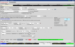
Actually, I have found several of IB’s own algos such as Scaletrader and Accumulate/Distribute to be very effective. Certainly IB seems very proud of them – IB CEO Thomas Peterffy has patented at least one of them. Accumulate/Distribute, for instance, is quite sophisticated, allowing the user to randomize and slice the size and interval between individual orders, use passive or aggressive order types, and pause execution on a news alert, or when the price falls below a moving average, or outside a specified range.

There is much to be said for using algos native to the execution platform rather than reinventing the wheel, providing the cost is reasonable. So, while it is perfectly feasible to build execution algos in Matlab, it typically isn’t necessary – in most cases standard algos will suffice.

There are exceptions, of course.  IB doesn’t offer the  kind of basket-trading capabilities REDIthat are available in advanced algo platforms like Tethys or RediPlus.  In those systems, for example, you can set the level of long/short imbalance in the portfolio that you are willing to tolerate and the algo will speed up or slow down execution of trades in individual components of the basket to maintain the dollar imbalance within that tolerance.  You can also manage the sector risk dynamically during execution.
Those kind of advanced capabilities don’t come cheap and you wont find them at IB, or any other retail platform. If you need that kind of functionality, for example, because you are trading a long/short equity portfolio within a universe of 200-300 names, your best option is probably to switch to a different execution platform.  Otherwise you will need to code a custom algo in your language of choice.

For many quantitative strategies, (at least the low frequency ones) IB’s standard algos are often good enough.  The Accumulate/Distribute algo, for instance, will show a visual representation of the progress of the execution of individuals legs of a pairs trade, and it is easy enough to identify a potential imbalance and adjust the algo parameters in real time. If you are only trading pairs, or small portfolios of cointegrated securities, it probably isn’t worthwhile to develop the sophisticated logic that would be required to handle the adjustment of the execution of individual legs of a trade in a fully automated way.  A large portfolio would be a different matter, however.

MATLAB EXAMPLE

I thought it might be instructive to take a look at how you might implement the execution of a strategy in Matlab, using IB algos. In the Matlab code fragment below, the (2 x nTickers) array tradeActions contains, in the first row, the action we wish to take (1 = BUY, -1 = SELL, -2 = SELL SHORT) and in the second row the (absolute value of) the number of shares we wish to trade for tickers i =1:nTickers. We break each order up into hundred lots and odd lots, routing the former via IB’s Accumulate/Distribute algo and the latter as passive REL orders (note that A/D  will typically randomize the timing of each sub-order, while REL orders are posted directly into the market). The Matlab function AccumulateDistribute implements the most important features of IB’s A/D algo, including random size and time slicing of the order.  Orders are submitted as passive REL orders with zero offset (so they will sit on the current bid or ask) – obviously you would typically want to consider allowing some non-zero offset for less liquid securities.  It is not hard to envisage how one might further enhance the algo to monitor the progress of the execution and speed up or slow down certain orders accordingly.

MatlabA couple of IB api “gotchas” to be aware of:

(i) IB requires unique and monotonically increasing orderIds for each order. One way to do this, suggested by Yair, is to use orderId = round((now-735000)*3e5);  This fails when you are submitting a number of orders sequentially at high speed (say in a for loop), where the time increments are sub-second, so you need to pass the orderID back and force a minimal increment, as I have in the code below.

(ii) It is very important to specify the primary exchange of each security:  securities with identical tickers can be found trading on different exchanges.  Failing to specify the primary exchange in such a case will result in IB rejecting the order with a typically cryptic api message.
Continue reading “Algorithmic Trading”

Equity Curve Money Management

Amongst a wide variety of money management methods that have evolved over the years, a perennial favorite is the use of the equity curve to guide position sizing.  The most common version of this technique is to add to the existing position (whether long or short) depending on the relationship between the current value of the account equity (realized + unrealized PL) and its moving average.  According to whether you believe that the  equity curve is momentum driven, or mean reverting, you will add to your existing position when the equity move above (or, on the case of mean-reverting, below) the long term moving average.

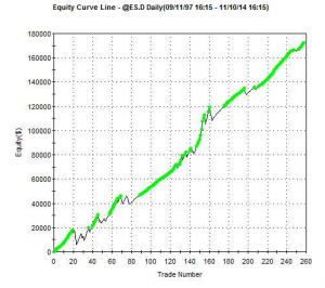
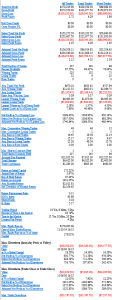
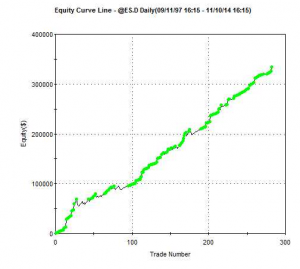
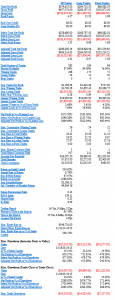
In this article I want to discuss a  slightly different version of equity curve money management, which is mean-reversion oriented.  The underlying thesis is that your trading strategy has good profit characteristics, and while it suffers from the occasional, significant drawdown, it can be expected to recover from the downswings.  You should therefore be looking to add to your positions when the equity curve moves down sufficiently, in the expectation that the trading strategy will recover.  The extra contracts you add to your position during such downturns  with increase the overall P&L. To illustrate the approach I am going to use a low frequency strategy on the S&P500 E-mini futures contract (ES).  The performance of the strategy is summarized in the chart and table below. EC PNL

(click to enlarge)

The overall results of the strategy are not bad:  at over 87% the  win rate is high as, too, is the profit factor of 2.72.  And the strategy’s performance, although hardly stellar, has been quite consistent over the period from 1997.  That said, most  the profits derive from the long side, and the strategy suffers from the occasional large loss, including a significant drawdown of over 18% in 2000.

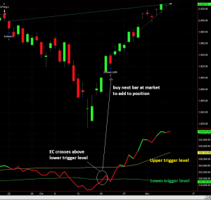
I am going to use this underlying strategy to illustrate how its performance can be improved with equity curve money management (ECMM).  To start, we calculate a simple moving average of the equity curve, as before.  However, in this variation of ECMM we then calculate offsets  that are a number of standard deviations above or below the moving average.  Typical default values for the moving average length might be 50 bars for a daily series, while we might  use, say,  +/- 2 S.D. above and below the moving average as our trigger levels. The idea is that we add to our position when the equity curve falls below the lower threshold level (moving average – 2x S.D) and then crosses back above it again.  This is similar to how a trader might use Bollinger bands, or an oscillator like Stochastics.  The chart below illustrates the procedure.

ED.D Chart with ECMM

The lower and upper trigger levels are shown as green and yellow lines in the chart indicator (note that in this variant of ECMM we only use the lower level to add to positions).

After a significant drawdown early in October the equity curve begins to revert and crosses back over the lower threshold level on Oct 21.  Applying our ECMM rule, we add to our existing long position the next day, Oct 22 (the same procedure would apply to adding to short positions).  As you can see, our money management trade worked out very well, since the EC did continue to mean-revert as expected. We closed the trade on Nov 11, for a substantial, additional profit.

Now we have illustrated the procedure, let’s being to explore the potential of the ECMM idea in more detail.  The first important point to understand is what ECMM will NOT do: i.e. reduce risk.  Like all money management techniques that are designed to pyramid into positions, ECMM will INCREASE risk, leading to higher drawdowns.  But ECMM should also increase profits:  so the question is whether the potential for greater profits is sufficient to offset the risk of greater losses.  If not, then there is a simpler alternative method of increasing profits: simply increase position size!  It follows that one of the key metrics of performance to focus on in evaluating this technique is the ratio of PL to drawdown.  Let’s look at some examples for our baseline strategy.

Single Entry, 2SD

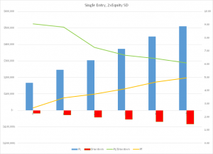
The chart shows the effect of adding a specified number of contracts to our existing long or short position whenever the equity curve crosses back above the lower trigger level, which in this case is set at 2xS.D below the 50-day moving average of the equity curve.  As expected, the overall strategy P&L increases linearly in line with the number of additional contracts traded, from a base level of around $170,000, to over $500,000 when we trade an additional five contracts.  So, too, does the profit factor rise from around 2.7 to around 5.0. That’s where the good news ends. Because, just as the strategy PL increases, so too does the size of the maximum drawdown, from $(18,500) in the baseline case to over $(83,000) when we trade an additional five contracts.  In fact, the PL/Drawdown ratio declines from over 9.0 in the baseline case, to only 6.0 when we trade the ECMM strategy with five additional contracts.  In terms of risk and reward, as measured by the PL/Drawdown ratio, we would be better off simply trading the baseline strategy:  if we traded 3 contracts instead of 1 contract, then without any money management at all we would have made total profits of around $500,000, but with a drawdown of just over $(56,000).  This is the same profit as produced with the 5-contract ECMM strategy, but with a drawdown that is $23,000 smaller.

SSALGOTRADING AD

How does this arise?  Quite simply, our ECMM money management trades as not all automatic winners from the get-go (even if they eventually produce profits.  In some cases, having crossed above the lower threshold level, the equity curve will subsequently cross back down below it again.  As it does so, the additional contracts we have traded are now adding to the strategy drawdown.

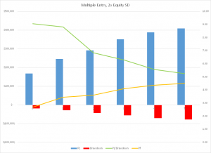
This suggests that there might be a better alternative.  How about if, instead of doing a single ECMM trade for, say, 5 additional contracts, we instead add an additional contract each time the equity curve crosses above the lower threshold level.  Sure, we might give up some extra profits, but our drawdown should be lower, right? That turns out to be true.  Unfortunately, however, profits are impacted more than the drawdown, so as a result the PL/Drawdown ratio shows the same precipitous decline:

Multiple Entry, 2SD

Once again, we would be better off trading the baseline strategy in larger size, rather than using ECMM, even when we scale into the additional contracts.

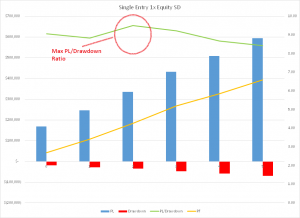
What else can we try?  An obvious trick to try is tweaking the threshold levels.  We can do this by adjusting the # of standard deviations at which to set the trigger levels.  Intuitively, it might seem that the obvious thing to do is set the threshold levels further apart, so that ECMM trades are triggered less frequently.  But, as it turns out, this does not produce the desired effect.  Instead, counter-intuitively, we have to set the threshold levels CLOSER to the moving average, at only +/-1x S.D.  The results are shown in the chart below.

Single Entry, 1SD

With these settings, the strategy PL and profit factor increase linearly, as before.  So too does the strategy drawdown, but at a slower rate.  As a consequence, the PL/Drawdown ration actually RISES, before declining at a moderate pace.  Looking at the chart, it is apparent the optimal setting is trading two additional contracts with a threshold setting one standard deviation below the 50-day moving average of the equity curve.

Below are the overall results.  With these settings the baseline strategy plus ECMM produces total profits of $334,000, a profit factor of 4.27 and a drawdown of $(35,212), making the PL/Drawdown ratio 9.50.  Producing the same rate of profits using the baseline strategy alone would require us to trade two contracts, producing a slightly higher drawdown of almost $(37,000).  So our ECMM strategy has increased overall profitability on a risk-adjusted basis.

EC with ECMM PNL ECMM

(Click to enlarge)

CONCLUSION

It is certainly feasible to improve not only the overall profitability of a strategy using equity curve money management, but also the risk-adjusted performance.  Whether ECMM will have much effect depends on the specifics of the underlying strategy, and the level at which the ECMM parameters are set to.  These can be optimized on a walk-forward basis.

EASYLANGUAGE CODE

Inputs:

MALen(50),
SDMultiple(2),
PositionMult(1),
ExitAtBreakeven(False);

Var:
OpenEquity(0),
EquitySD(0),
EquityMA(0),
UpperEquityLevel(0),
LowerEquityLevel(0),
NShares(0);

OpenEquity=OpenPositionProfit+NetProfit;a
EquitySD=stddev(OpenEquity,MALen);
EquityMA=average(OpenEquity,MALen);
UpperEquityLevel=EquityMA + SDMultiple*EquitySD;
LowerEquityLevel=EquityMA-SDMultiple*EquitySD;
NShares=CurrentContracts*PositionMult;
If OpenEquity crosses above LowerEquityLevel then begin
If Marketposition > 0 then begin
Buy(“EnMark-LMM”) NShares shares next bar at market;
end;
If Marketposition < 0 then begin
Sell Short(“EnMark-SMM”) NShares shares next bar at market;
end;
end;
If ExitAtBreakeven then begin

If OpenEquity crosses above EquityMA then begin
If Marketposition > 1 then begin
Sell Short (“ExBE-LMM”) (Currentcontracts-1) shares next bar at market;
end;
If Marketposition < -1 then begin
Buy (“ExBE-SMM”) (Currentcontracts-1) shares next bar at market;
end;

end;
end;

A Calendar Spread Strategy in VIX Futures

I have been working on developing some high frequency spread strategies using Trading Technologies’ Algo Strategy Engine, which is extremely impressive (more on this in a later post).  I decided to take a time out to experiment with a slower version of one of the trades, a calendar spread in VIX futures that trades  the spread on the front two contracts.  The strategy applies a variety of trend-following and mean-reversion indicators to trade the spread on a daily basis.

Modeling a spread strategy on a retail platform like Interactivebrokers or TradeStation is extremely challenging, due to the limitations of the platform and the Easylanguage programming language compared to professional platforms that are built for purpose, like TT’s XTrader and development tools like ADL.  If you backtest strategies based on signals generated from the spread calculated using the last traded prices in the two securities, you will almost certainly see “phantom trades” – trades that could not be executed at the indicated spread price (for example, because both contracts last traded on the same side of the bid/ask spread).   You also can’t easily simulate passive entry or exit strategies, which typically constrains you to using market orders for both legs, in and out of the spread.  On the other hand, while using market orders would almost certainly be prohibitively expensive in a high frequency or daytrading context, in a low-frequency scenario the higher transaction costs entailed in aggressive entries and exits are typically amortized over far longer time frames.

SSALGOTRADING AD

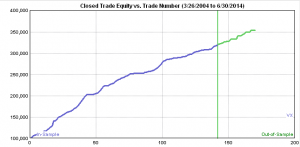
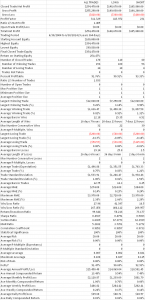
In the following example I have allowed transaction costs of $100 per round turn and slippage of $0.1 (equivalent to $100) per spread.  Daily settlement prices from Mar 2004 to June 2010 were used to fit the model, which was tested out of sample in the period July 2010 to June 2014. Results are summarized in the chart and table below.

Even burdened with significant transaction cost assumptions the strategy performance looks impressive on several counts, notably a profit factor in excess of 300, a win rate of over 90% and a Sortino Ratio of over 6.  These features of the strategy prove robust (and even increase) during the four year out-of-sample period, although the annual net profit per spread declines to around $8,500, from $36,600 for the in-sample period.  Even so, this being a straightforward calendar spread, it should be possible to trade the strategy in size at relative modest margin cost, making the strategy return highly attractive.

Equity Curve

 (click to enlarge)

Performance Results


(click to enlarge)


A Scalping Strategy in E-Mini Futures

This is a follow up post to my post on the Mathematics of Scalping. To illustrate the scalping methodology, I coded up a simple strategy based on the techniques described in the post.

The strategy trades a single @ES contract on 1-minute bars. The attached ELD file contains the Easylanguage code for ES scalping strategy, which can be run in Tradestation or Multicharts.

This strategy makes no attempt to forecast market direction and doesn’t consider market trends at all. It simply looks at the current levels of volatility and takes a long volatility position or a short volatility position depending on whether volatility is above or below some threshold parameters.

By long volatility I mean a position where we buy or sell the market and set a loose Profit Target and a tight Stop Loss. By short volatility I mean a position where we buy or sell the market and set a tight Profit Target and loose Stop Loss. This is exactly the methodology I described earlier in the post. The parameters I ended up using are as follows:

Long Volatility: Profit Target = 8 ticks, Stop Loss = 2 ticks
Short Volatility: Profit Target = 2 ticks, Stop Loss = 30 ticks

I have made no attempt to optimize these parameters settings, which can easily be done in Tradestation or Multicharts.

What do we mean by volatility being above our threshold level? I use a very simple metric: I take the TrueRange for the current bar and add 50% of the increase or decrease in TrueRange over the last two bars. That’s my crude volatility “forecast”.

SSALGOTRADING AD

The final point to explain is this: let’s suppose our volatility forecast is above our threshold level, so we know we want to be long volatility. Ok, but do we buy or sell the ES? One approach ia to try to gauge the direction of the market by estimating the trend. Not a bad idea, by any means, although I have argued that volatility drowns out any trend signal at short time frames (like 1 minute, for example). So I prefer an approach that makes no assumptions about market direction.

In this approach what we do is divide volatility into upsideVolatility and downsideVolatility. upsideVolatility uses the TrueRange for bars where Close > Close[1]. downsideVolatility is calculated only for bars where Close < Close[1]. This kind of methodology, where you calculate volatility based on the sign of the returns, is well known and is used in performance measures like the Sortino ratio. This is like the Sharpe ratio, except that you calculate the standard deviation of returns using only days in which the market was down. When it’s calculated this way, standard deviation is known as the (square root of the) semi-variance.

Anyway, back to our strategy. So we calculate the upside and downside volatilities and test them against our upper and lower volatility thresholds.

The decision tree looks like this:

LONG VOLATILITY
If upsideVolatilityForecast > upperVolThrehold, buy at the market with wide PT and tight ST (long market, long volatility)
If downsideVolatilityForecast > upperVolThrehold, sell at the market with wide PT and tight ST (short market, long volatility)

SHORT VOLATILITY
If upsideVolatilityForecast < lowerVolThrehold, sell at the Ask on a limit with tight PT and wide ST (short market, short volatility)
If downsideVolatilityForecast < lowerVolThrehold, buy at the Bid on a limit with tight PT and wide ST (long market, short volatility)

NOTE THE FOLLOWING CAVEATS. DO NOT TRY TO TRADE THIS STRATEGY LIVE (but use it as a basis for a tradable strategy)

1. The strategy makes the usual TS assumption about fill rates, which is unrealistic, especially at short intervals like 1-minute.
2. The strategy allows fees and commissions of $3 per contract, or $6 per round turn. Your trading costs may be higher than this.
3. Tradestation is unable to perform analysis at the tick level for a period as long at the one used here (2000 to 2014). A tick by tick analysis would likely show very different results (better or worse).
4. The strategy is extremely lop-sided: the great majority of the profits are made on the long side and the Win Rates and Profit Factors are very different for long trades vs short trades. I suspect this would change with a tick by tick analysis. But it also may be necessary to add more parameters so that long trades are treated differently from short trades.
5. No attempt has been made to optimize the parameters.
6 This is a daytading strategy that will exit the market on close.

So with all that said here are the results.

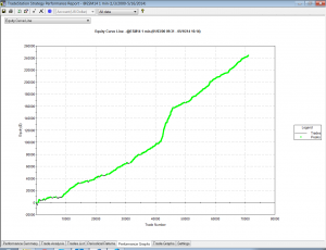
As you can see, the strategy produces a smooth, upward sloping equity curve, the slope of which increases markedly during the period of high market volatility in 2008.
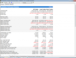
Net profits after commissions for a single ES contract amount to $243,000 ($3.42 per contract) with a win rate of 76% and Profit Factor of 1.24.

This basic implementation would obviously require improvement in several areas, not least of which would be to address the imbalance in strategy profitability on the short vs long side, where most of the profits are generated.

Scalping Strategy EC


Scalping Strategy Perf Report


How to Spot a Fake

One of the issues that comes up regularly is how, as an investor or other interested party, one can protect oneself from unscrupulous scam artists posing as professional traders or money managers. This is a particular problem on web sites featuring trader forums, where individuals with unverified track records claiming stellar trading histories use their purported trading “prowess” to try to impress and intimidate other participants, usually impressionable newbies. The purpose of this post is to provide some guidance to help investors, traders and other fellow travelers sort the wheat from the chaff. We’ll be doing some forensic analysis on the track record for a strategy in NG futures that one such character recently posted in one of these forums, as a classic example of the kind of fakery I am describing.

One thing you should understand about scam artists operating on forums, is that they don’t work alone: usually they have a bunch of groupies who will shill for them at every opportunity and who will try to shout down any investigative questioning. Don’t be deterred. These know-it-alls are usually just ignorant dupes, who understand no more about trading than the scam artist. They may just as easily be fellow-scam artists themselves.

THE FIRST BIG RED FLAG: UNWILLINGNESS TO PRODUCE A TRACK RECORD
Anyone claiming to be a CTA or professional money manager (or whose shills claim he is one) has to have a track record that is freely available in the public domain. So how does a scam artist overcome a challenge to produce it? He will claim that he “can’t advertise”, or make some other, similar excuse. Don’t accept that at face value. Ask him to PM it to you. If he won’t, there’s already a high probability he’s a con artist.

THE SECOND BIG RED FLAG: CURVE FITTING
Let’s say our suspect meets the challenge and produces a track record. Ideally this will be an audited P&L statement, but let’s assume for the purposes of this discussion that he produces something along the lines of the Performance Reports produced by a product like Tradestation or MultiCharts, i.e. we are dealing with a simulated back-test.

If your suspect produces a back-test, you can be pretty sure it’s going to look good – otherwise he wouldn’t produce it. The task now is to dig into those reports to spot the red flags that give clues as to whether it might be fake.
Now of course any trading system is going to make assumptions – about fill rates, slippage, commissions, capacity etc. All that is fine, as long as the assumptions are clearly stated. You might want to challenge any or all of the assumptions, and the trader may disagree with you about some or all of them. That’s perfectly ok – it’s an honest, open discussion about a set of investment assumptions that have been revealed at the outset.

But here is what is NOT ok: any opacity about which data was used to build the trading model and which data was used to test it. The former, the in-sample (IS) data set, used to construct the model, must be entirely separate and distinct from the out-of-sample (OOS) data set. It is trivially easy using a tool like Tradestation to produce a trading system that shows stellar results in-sample, but which will immediately crash and burn when it is used in live trading. This is known as curve-fitting. And it’s by far the most common method by which scam artists try to dupe investors.

In order to demonstrate the robustness of the system prior to risking real money, a genuine trader will test his system OOS and show you the results. What you are looking for ideally is congruity between the IS and OOS results. Now by congruity, I don’t mean that they should be identical. Far from it – markets evolve and strategy performance will vary over time. But what you are hoping is that the key performance metrics in the OOS and IS periods, such as annual returns, Sharpe ratio, PNL per contract, profit ratio and win rate, will be comparable. At the very least, you would like to be able to identify some portion of the IS data set for which the strategy performance characteristics are similar to those in the OOS period.

Any – I mean ANY – ambiguity or lack of clarity about which data was used to build the model and which was used for OOS testing is a HUGE red flag. Chances are, your scam artist is already trying to fudge the issue that he curve-fitted the system.
This was the case in the recent forum post we are using as a test case. The trader made no attempt whatsoever to clarify which data was used for model development and which for testing. Immediately, I was suspicious and began looking for other evidence of curve fitting. It didn’t take me long to find it.

THE THIRD BIG RED FLAG: THE EQUITY CURVE
The first item I turned to in the performance reports was the equity curve and I immediately spotted two rather large clues that I was dealing with a fake.

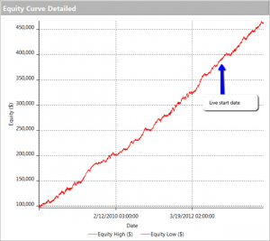
The first clue was the large sign on the chart labelled “live start date”. What does this mean? This is a back-test, so all of the results are theoretical, including those after the supposed “live start date” sometime in 2013. What the faker is trying to do is imply the part of the equity curve shown after that date indicate actual performance results. He doesn’t actually claim this, so he has plausible deniability if you call him on it (“I said it was just a back test”). But he hopes that you won’t, and that, by default, you’ll accept these results are real. But they aren’t.

The second clue of fakery is much more important: the equity curve itself. When someone shows you and equity curve like the one reported by this trader, rising in a straight line from the lower left to upper right quadrants, you can be 99% confident that you are dealing with a fake.
You see, in finance there are almost never any straight lines. They are as rare as unicorns. Especially when it comes to strategy performance. They only time you will EVER see an equity curve like this is when you are looking at the equity curve of (i) a high frequency market making trading system or (ii) a fake, produced by curve fitting a strategy to the ENTIRE data set.
And this strategy was not high frequency – as we shall see, it operated on 15 minute bars, holding positions overnight.

EC Chart

THE FOURTH BIG RED FLAG: GOD’s EQUITY CURVE
I said that straight line equity curve were extremely rare. In fact, even God’s equity curve isn’t often a straight line. What does that mean?

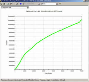
Suppose you had a strategy that could predict with 100% accuracy whether the market would go up or down over the next bar (whether you are using daily bars, or 15 minute bars, as in our example). The system would buy (or hold) when the market was forecast to rise, and sell when the market was predicted to fall. What would the performance of such a perfect system look like? Pretty stellar, obviously. And most people would guess that the system’s equity curve would be a straight line, or maybe even exponential in shape. In fact that’s typically not the case. God’s equity curve will be sloped and kinked, just like any other equity curve. And if your suspect’s equity curve is real, it should show some commonality with God’s equity curve, by which I mean it should show changes in slope and level that reflect those seen in the perfect equity curve.

What does God’s Equity Curve look like in NG futures?

Gods EC

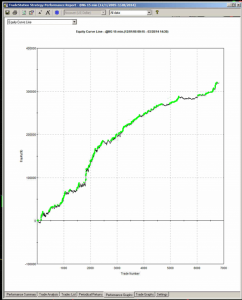
As you can see it’s not straight. In fact it’s concave. So a REAL equity curve should have similar characteristics, like this one, for example:

NG EC

As you can see, the equity curve of the real trading system track’s God’s Equity Curve, albeit at a much lower level. It’s concave, with an upswing during the final few months of trading, just like God’s. That’s a good sign that the strategy back-test is very likely genuine (which it is – I produced it).

Why is Gods’ Equity Curve the shape it is? The answer will vary from market to market. In the case of NG, the suggestion is that the market is becoming more efficient: simple trading strategies based on technical indicators work less well than they did five years ago. We have seen something very similar in F/X markets. During the 1970’s and 1980’s when Soros was active in the field, simple strategies like moving average crossovers made great returns, but these entirely dissipated in the 1990’s, with the advent of widely available computing power.

THE FIFTH BIG RED FLAG: THE SHILL SHOUTDOWN
When I posted my analysis, which clearly indicated fakery by this well known forum participant, I was immediately flamed by one of his supporters who shouted something to the effect that (i) everyone knows that the downward slope of God’s Equity Curve was caused by volatility and (ii) the star trader, unlike God, or me, knows about position sizing.

This attempt at misdirection in the face of awkward facts is a classic sign of fakery. What distinguishes the shill post is:

(i) Immediacy – clearly no attempt has been made to evaluate the argument or analysis. The shill simply attempts to drown out the critic with a lot of noise, as quickly as possible.

(ii) Plausibility – shills will throw around terms that lend plausibility to their objection, but which after a moment’s reflection are entirely irrelevant or, as in this case, detrimental to their own cause.

(iii) Invective – the more intemperate the post, the more likely the shill is simply trying to provide cover for the faker.

So let’s take a moment to dispose of the plausible sounding objections posted by the shill in this example.
I am going to take it as read that everyone understands that trading profitability is positively correlated with volatility. There is a huge amount of empirical research supporting that finding, but to keep it simple we can appeal to one of the cornerstones of modern finance: risk and return. The higher the volatility, i.e. the greater the risk, the greater the return traders and investors in the markets will require on their capital. This is a principle of modern financial theory that even a graduate of the Scranton college of fine art should be expected to appreciate.

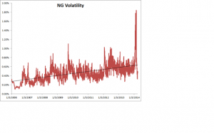
So what’s the story with NG volatility? You can see the time series of NG volatility in the chart below. One feature stands out above all others: the upward slope of the curve. NG volatility has RISEN over the sample period from 2008 to 2014. Consequently, returns from trading NG futures should also have RISEN rather than fallen. One thing we can say for sure, whatever caused the concave shape in God’s Equity Curve in NG futures, it was NOT volatility!

NG Volatility

Turning to the shill’s next, plausible sounding, but dubious “explanation”, position sizing: this really is completely irrelevant. Because, as we shall see from an examination of the performance report, the track record was created by trading a constant one-lot! So this was just an attempt to sound “sophisticated” by someone trying to misdirect the reader away from the increasingly obvious evidence of fakery.

THE SIXTH BIG RED FLAG: LOW DRAWDOWNS AND OVERNIGHT GAP RISK
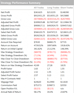
One of the highly unusual features of our faker’s equity curve is it’s exceptional smoothness. Low volatility in the equity curve is, in and of itself, an indicator the track record results from curve fitting. But we can get even more insight by digging into the performance report, shown below.

Perf 1
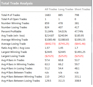
Perf 2

As you can see from the second page of the report, the strategy holds positions for an average of 57 15-minute bars, equivalent to slightly over 14 hours. So this is a low frequency strategy that takes overnight risk. Now, as any trader will know, overnight gap risk in a product like NG can be very significant and likely to be produce much larger drawdowns over a 5 year period than the $8,470 reported here.

The only other possible explanation is that the strategy is traded continuously through both day and night sessions. But this is not only itself improbable, it gives rise to another implausibility: liquidity in the overnight session is so poor that the strategy is unlikely to be able to trade more than 1-2 contracts, at most. This would be of little value to a CTA, or its customers, whatever the star trader’s protestations that his “clients are happy”.

There is no plausible way to resolve the disconnection between the low drawdown, overnight gap risk and market illiquidity. The most plausible explanation: the back-test is a curve fitting exercise.

THE SEVENTH AN FINAL BIG RED FLAG: INCONSISTENCY BETWEEN PERFORMANCE METRICS
As any experienced strategy developer knows, you can get some of the things you want, but you can never achieve all of them. Amongst the desirable features to be maximized are
• Profit factor
• Average PNL per contract
• Percentage win rate

There is a trade-off between the features. A high PNL per contract typically means you are trading less frequently, with longer hold periods, and consequently the percentage win rate tends to be lower. Alternatively, you can increase the win rate, at the cost of lowering the average PNL per contract and/or the profit factor. And so on.

This strategy purports to have it all: a high average PNL per contract resulting from low frequency trading, coupled with good percentage win rate of over 50% and profit factor. A win rate of much over 40% is highly unusual for a momentum strategy entering and exiting with market or stop orders – and its almost inconceivable for a strategy with a PNL per contract and profit factor as large as suggested here.

CONCLUSION
This back-test fails the sniff test on so many levels, I would rate the chance of it being real as less than 1 in 1000.
The final, conclusive proof of fakery is that the “star trader” responsible for producing the report was unable and/or unwilling to attempt to answer even a single one of the criticisms.

So, be warned. If you see forum members banding about track records like this one, you can be sure that they and their strategies are likely to be fake, and not to be trusted.