Scalping vs. Market Making
A market-making strategy is one in which the system continually quotes on the bid and offer and looks to make money from the bid-offer spread (and also, in the case of equities, rebates). During a typical trading day, inventories will build up on the long or short side of the book as the market trades up and down. There is no intent to take a market view as such, but most sophisticated market making strategies will use microstructure models to help decide whether to “lean” on the bid or offer at any given moment. Market makers may also shade their quotes to reduce the buildup of inventory, or even pull quotes altogether if they suspect that informed traders are trading against them (a situation referred to as “toxic flow”). They can cover short positions through the repo desk and use derivatives to hedge out the risk of an accumulated inventory position.
A scalping strategy shares some of the characteristics of a market making strategy: it will typically be mean reverting, seeking to enter passively on the bid or offer and the average PL per trade is often in the region of a single tick. But where a scalping strategy differs from market making is that it does take a view as to when to get long or short the market, although that view may change many times over the course of a trading session. Consequently, a scalping strategy will only ever operate on one side of the market at a time, working the bid or offer; and it will typically never build inventory, since will it usually reverse and later try to sell for a profit the inventory it has previously purchased, hopefully at a lower price.
In terms of performance characteristics, a market making strategy will often have a double-digit Sharpe Ratio, which means that it may go for many days, weeks, or months, without taking a loss. Scalping is inherently riskier, since it is taking directional bets, albeit over short time horizons. With a Sharpe Ratio in the region of 3 to 5, a scalping strategy will often experience losing days and even losing months.
So why prefer scalping to market making? It’s really a question of capability. Competitive advantage in scalping derives from the successful exploitation of identified sources of alpha, whereas market making depends primarily on speed and execution capability. Market making requires HFT infrastructure with latency measured in microseconds, the ability to layer orders up and down the book and manage order priority. Scalping algos are generally much less demanding in terms of trading platform requirements: depending on the specifics of the system, they can be implemented successfully on many third party networks.
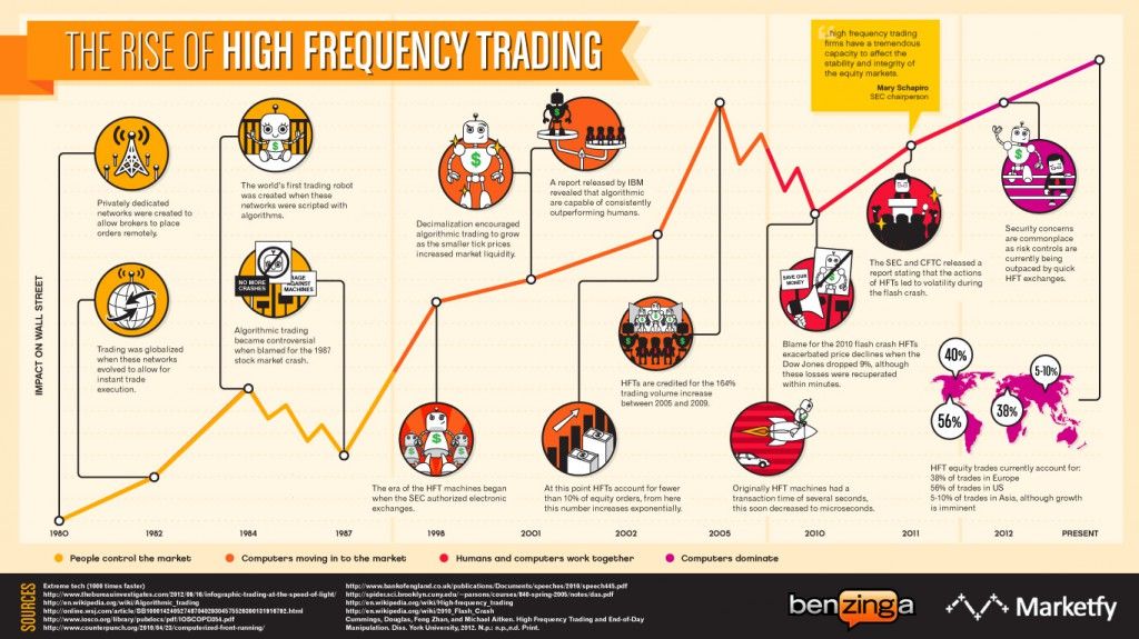
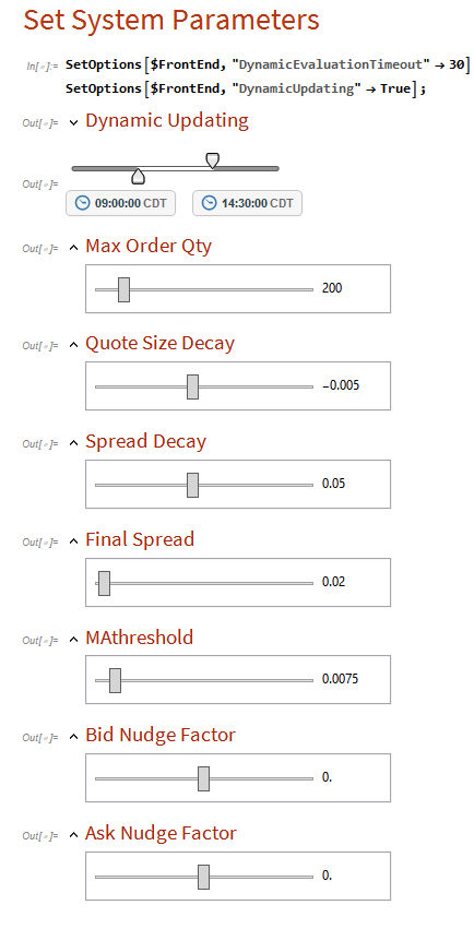
Developing HFT Futures Strategies
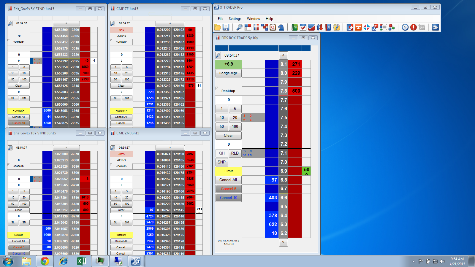
Some time ago my firm Systematic Strategies began research and development on a number of HFT strategies in futures markets. Our primary focus has always been HFT equity strategies, so this was something of a departure for us, one that has entailed a significant technological obstacles (more on this in due course). Amongst the strategies we developed were several very profitable scalping algorithms in fixed income futures. The majority trade at high frequency, with short holding periods measured in seconds or minutes, trading tens or even hundreds of times a day.
 The next challenge we faced was what to do with our research product. As a proprietary trading firm our first instinct was to trade the strategies ourselves; but the original intent had been to develop strategies that could provide the basis of a hedge fund or CTA offering. Many HFT strategies are unsuitable for that purpose, since the technical requirements exceed the capabilities of the great majority of standard trading platforms typically used by managed account investors. Besides, HFT strategies typically offer too limited capacity to be interesting to larger, institutional investors.
In the end we arrived at a compromise solution, keeping the highest frequency strategies in-house, while offering the lower frequency strategies to outside investors. This enabled us to keep the limited capacity of the highest frequency strategies for our own trading, while offering investors significant capacity in strategies that trade at lower frequencies, but still with very high performance characteristics.
HFT Bond Scalping
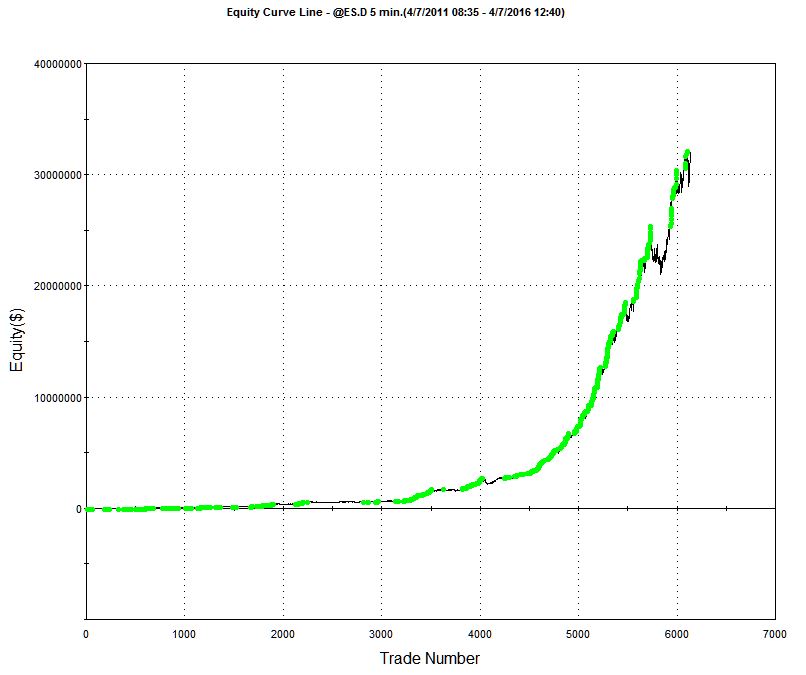
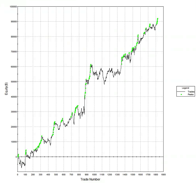
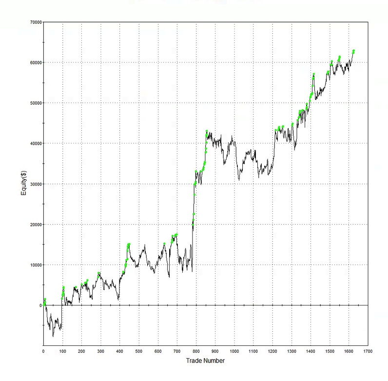
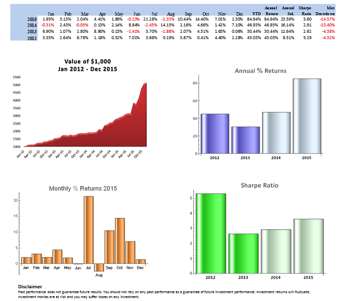
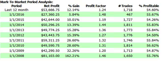
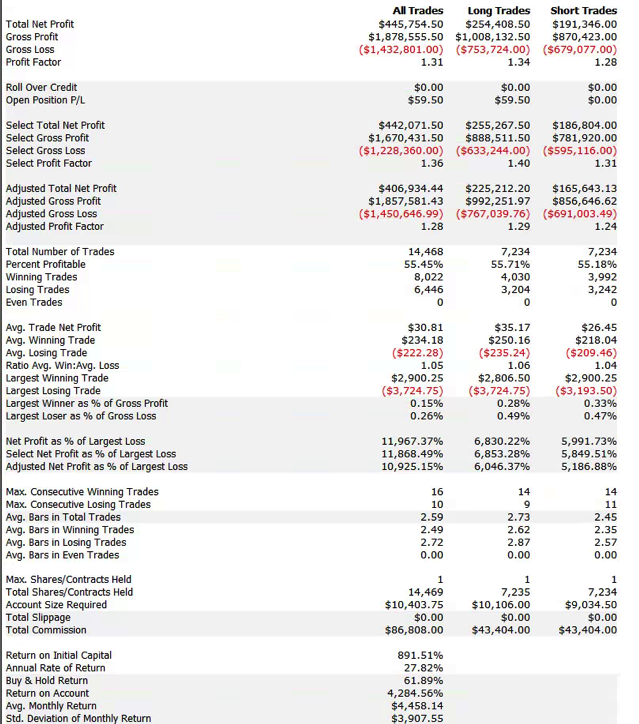
A typical example is the following scalping strategy in US Bond Futures. The strategy combines two of the lower frequency algorithms we developed for bond futures that scalp around 10 times per session. The strategy attempts to take around 8 ticks out of the market on each trade and averages around 1 tick per trade. With a Sharpe Ratio of over 3, the strategy has produced net profits of approximately $50,000 per contract per year, since 2008. A pleasing characteristic of this and other scalping strategies is their consistency: There have been only 10 losing months since January 2008, the last being a loss of $7,100 in Dec 2015 (the prior loss being $472 in July 2013!)
Annual P&L
Strategy Performance

Offering The Strategy to Investors on Collective2
The next challenge for us to solve was how best to introduce the program to potential investors. Systematic Strategies is not a CTA and our investors are typically interested in equity strategies. It takes a great deal of hard work to persuade investors that we are able to transfer our expertise in equity markets to the very different world of futures trading. While those efforts are continuing with my colleagues in Chicago, I decided to conduct an experiment: what if we were to offer a scalping strategy through an online service like Collective2? For those who are unfamiliar, Collective2 is an automated trading-system platform that allowed the tracking, verification, and auto-trading of multiple systems. The platform keeps track of the system profit and loss, margin requirements, and performance statistics. It then allows investors to follow the system in live trading, entering the system’s trading signals either manually or automatically.
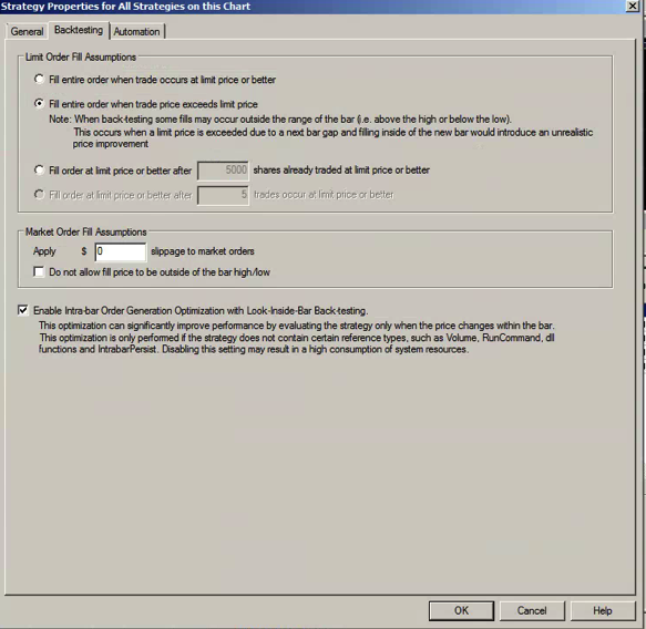
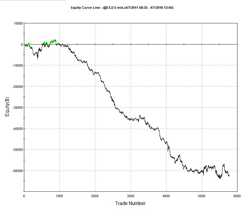
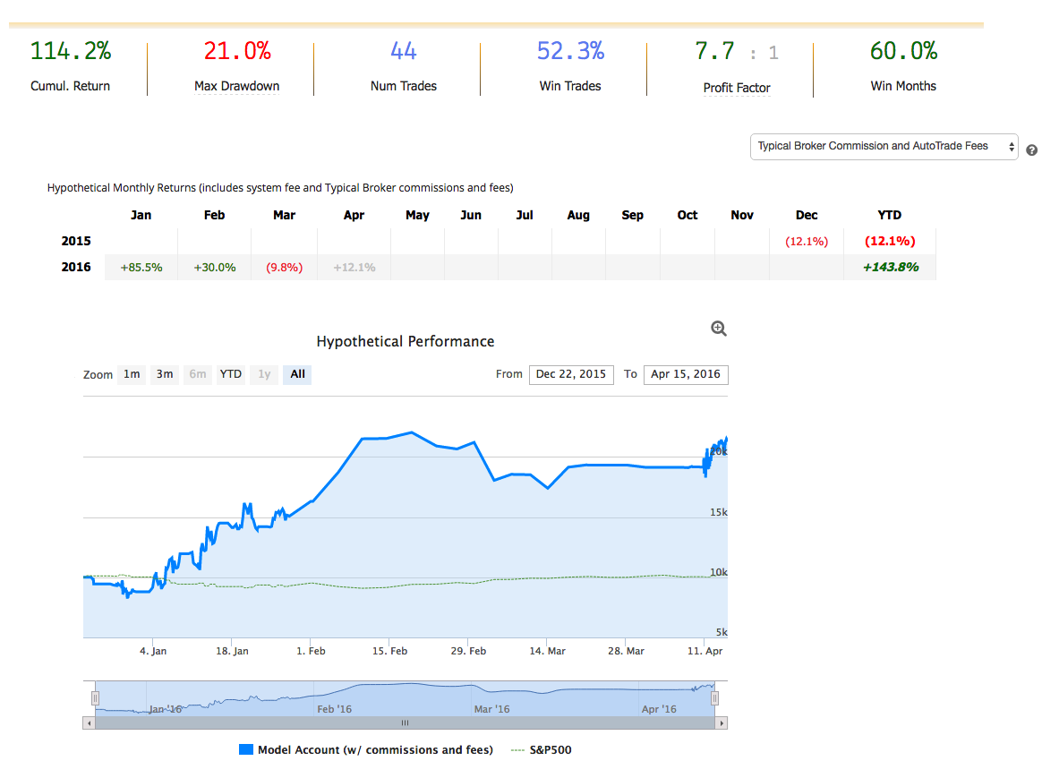
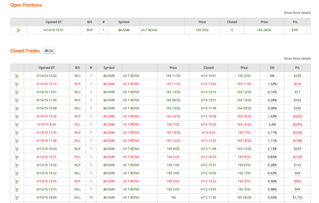
Offering a scalping strategy on a platform like this certainly creates visibility (and a credible track record) with investors; but it also poses new challenges. For example, the platform assumes trading cost of around $14 per round turn, which is at least 2x more expensive than most retail platforms and perhaps 3x-5x more expensive than the cost a HFT firm might pay. For most scalping strategies that are designed to take a tick out of the market such high fees would eviscerate the returns. This motivated our choice of US Bond Futures, since the tick size and average trade are sufficiently large to overcome even this level of trading friction. After a couple of false starts, during which we played around with the algorithms and boosted strategy profitability with a couple of low frequency trades, the system is now happily humming along and demonstrating the kind of performance it should (see below).
For those who are interested in following the strategy’s performance, the link on collective2 is here.
Disclaimer
About the results you see on this Web site
Past results are not necessarily indicative of future results.
These results are based on simulated or hypothetical performance results that have certain inherent limitations. Unlike the results shown in an actual performance record, these results do not represent actual trading. Also, because these trades have not actually been executed, these results may have under-or over-compensated for the impact, if any, of certain market factors, such as lack of liquidity. Simulated or hypothetical trading programs in general are also subject to the fact that they are designed with the benefit of hindsight. No representation is being made that any account will or is likely to achieve profits or losses similar to these being shown.
In addition, hypothetical trading does not involve financial risk, and no hypothetical trading record can completely account for the impact of financial risk in actual trading. For example, the ability to withstand losses or to adhere to a particular trading program in spite of trading losses are material points which can also adversely affect actual trading results. There are numerous other factors related to the markets in general or to the implementation of any specific trading program, which cannot be fully accounted for in the preparation of hypothetical performance results and all of which can adversely affect actual trading results.
Material assumptions and methods used when calculating results
The following are material assumptions used when calculating any hypothetical monthly results that appear on our web site.
- Profits are reinvested. We assume profits (when there are profits) are reinvested in the trading strategy.
- Starting investment size. For any trading strategy on our site, hypothetical results are based on the assumption that you invested the starting amount shown on the strategy’s performance chart. In some cases, nominal dollar amounts on the equity chart have been re-scaled downward to make current go-forward trading sizes more manageable. In these cases, it may not have been possible to trade the strategy historically at the equity levels shown on the chart, and a higher minimum capital was required in the past.
- All fees are included. When calculating cumulative returns, we try to estimate and include all the fees a typical trader incurs when AutoTrading using AutoTrade technology. This includes the subscription cost of the strategy, plus any per-trade AutoTrade fees, plus estimated broker commissions if any.
- “Max Drawdown” Calculation Method. We calculate the Max Drawdown statistic as follows. Our computer software looks at the equity chart of the system in question and finds the largest percentage amount that the equity chart ever declines from a local “peak” to a subsequent point in time (thus this is formally called “Maximum Peak to Valley Drawdown.”) While this is useful information when evaluating trading systems, you should keep in mind that past performance does not guarantee future results. Therefore, future drawdowns may be larger than the historical maximum drawdowns you see here.
Trading is risky
There is a substantial risk of loss in futures and forex trading. Online trading of stocks and options is extremely risky. Assume you will lose money. Don’t trade with money you cannot afford to lose.