A Scalping Strategy in E-Mini Futures

This is a follow up post to my post on the Mathematics of Scalping. To illustrate the scalping methodology, I coded up a simple strategy based on the techniques described in the post.

The strategy trades a single @ES contract on 1-minute bars. The attached ELD file contains the Easylanguage code for ES scalping strategy, which can be run in Tradestation or Multicharts.

This strategy makes no attempt to forecast market direction and doesn’t consider market trends at all. It simply looks at the current levels of volatility and takes a long volatility position or a short volatility position depending on whether volatility is above or below some threshold parameters.

By long volatility I mean a position where we buy or sell the market and set a loose Profit Target and a tight Stop Loss. By short volatility I mean a position where we buy or sell the market and set a tight Profit Target and loose Stop Loss. This is exactly the methodology I described earlier in the post. The parameters I ended up using are as follows:

Long Volatility: Profit Target = 8 ticks, Stop Loss = 2 ticks
Short Volatility: Profit Target = 2 ticks, Stop Loss = 30 ticks

I have made no attempt to optimize these parameters settings, which can easily be done in Tradestation or Multicharts.

What do we mean by volatility being above our threshold level? I use a very simple metric: I take the TrueRange for the current bar and add 50% of the increase or decrease in TrueRange over the last two bars. That’s my crude volatility “forecast”.

SSALGOTRADING AD

The final point to explain is this: let’s suppose our volatility forecast is above our threshold level, so we know we want to be long volatility. Ok, but do we buy or sell the ES? One approach ia to try to gauge the direction of the market by estimating the trend. Not a bad idea, by any means, although I have argued that volatility drowns out any trend signal at short time frames (like 1 minute, for example). So I prefer an approach that makes no assumptions about market direction.

In this approach what we do is divide volatility into upsideVolatility and downsideVolatility. upsideVolatility uses the TrueRange for bars where Close > Close[1]. downsideVolatility is calculated only for bars where Close < Close[1]. This kind of methodology, where you calculate volatility based on the sign of the returns, is well known and is used in performance measures like the Sortino ratio. This is like the Sharpe ratio, except that you calculate the standard deviation of returns using only days in which the market was down. When it’s calculated this way, standard deviation is known as the (square root of the) semi-variance.

Anyway, back to our strategy. So we calculate the upside and downside volatilities and test them against our upper and lower volatility thresholds.

The decision tree looks like this:

LONG VOLATILITY
If upsideVolatilityForecast > upperVolThrehold, buy at the market with wide PT and tight ST (long market, long volatility)
If downsideVolatilityForecast > upperVolThrehold, sell at the market with wide PT and tight ST (short market, long volatility)

SHORT VOLATILITY
If upsideVolatilityForecast < lowerVolThrehold, sell at the Ask on a limit with tight PT and wide ST (short market, short volatility)
If downsideVolatilityForecast < lowerVolThrehold, buy at the Bid on a limit with tight PT and wide ST (long market, short volatility)

NOTE THE FOLLOWING CAVEATS. DO NOT TRY TO TRADE THIS STRATEGY LIVE (but use it as a basis for a tradable strategy)

1. The strategy makes the usual TS assumption about fill rates, which is unrealistic, especially at short intervals like 1-minute.
2. The strategy allows fees and commissions of $3 per contract, or $6 per round turn. Your trading costs may be higher than this.
3. Tradestation is unable to perform analysis at the tick level for a period as long at the one used here (2000 to 2014). A tick by tick analysis would likely show very different results (better or worse).
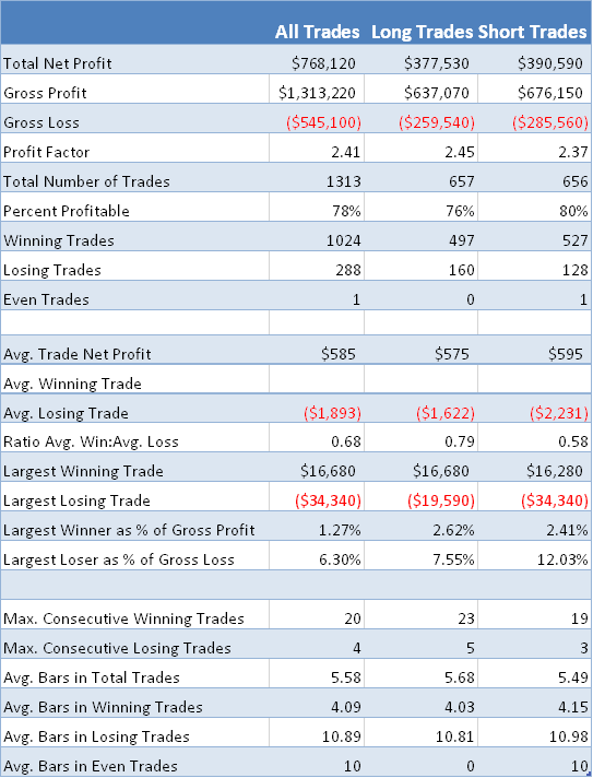
4. The strategy is extremely lop-sided: the great majority of the profits are made on the long side and the Win Rates and Profit Factors are very different for long trades vs short trades. I suspect this would change with a tick by tick analysis. But it also may be necessary to add more parameters so that long trades are treated differently from short trades.
5. No attempt has been made to optimize the parameters.
6 This is a daytading strategy that will exit the market on close.

So with all that said here are the results.

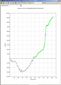
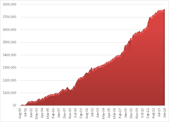
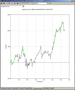
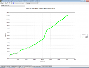
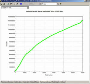
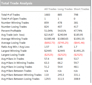
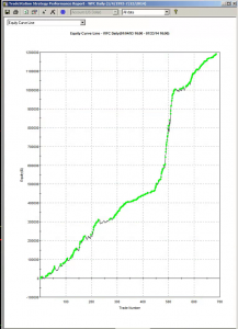
As you can see, the strategy produces a smooth, upward sloping equity curve, the slope of which increases markedly during the period of high market volatility in 2008.
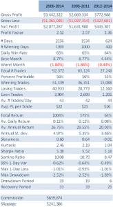
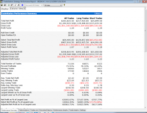
Net profits after commissions for a single ES contract amount to $243,000 ($3.42 per contract) with a win rate of 76% and Profit Factor of 1.24.

This basic implementation would obviously require improvement in several areas, not least of which would be to address the imbalance in strategy profitability on the short vs long side, where most of the profits are generated.

Scalping Strategy EC


Scalping Strategy Perf Report


Quantitative Analysis of Fat Tails – JonathanKinlay.com

In this quantitative analysis I explore how, starting from the assumption of a stable, Gaussian distribution in a returns process, we evolve to a system that displays all the characteristics of empirical market data, notably time-dependent moments, high levels of kurtosis and fat tails.  As it turns out, the only additional assumption one needs to make is that the market is periodically disturbed by the random arrival of news.

NOTE:  if you are unable to see the Mathematica models below, you can download the free Wolfram CDF player and you may also need this plug-in.

You can also download the complete Mathematica CDF file here.

Stationarity

A stationary process is one that evolves over time, but whose probability distribution does not vary with time. As the word implies, such a process is stable. More formally, the moments of the distribution are independent of time.

Let’s assume we are dealing with such a process that have constant mean μ and constant volatility (standard deviation) σ.

 Φ=NormalDistribution[μ,σ]

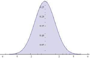
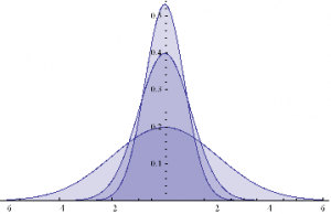
Here are some examples of Normal probability distributions, with constant mean μ = 0 and standard deviation σ ranging from 0.75 to 2

 Plot[Evaluate@Table[PDF[Φ,x],{σ,{.75,1,2}}]/.μ→0,{x,-6,6},Filling→Axis]


Chart 1

The moments of Φ are given by:

 Through[{Mean, StandardDeviation, Skewness, Kurtosis}[Φ]]

{μ,  σ,  0,   3}

They, too, are time – independent.

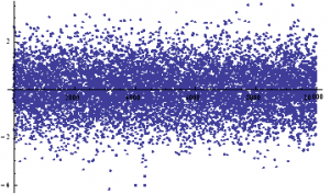
We can simulate some observations from such a process, with, say, mean μ = 0 and standard deviation σ = 1:

ListPlot[sampleData=RandomVariate[Φ /.{μ→0, σ→1},10^4]]


Chart 2

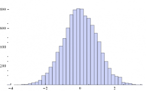
Histogram[sampleData]

Chart 3

If we assume for the moment that such a process is an adequate description of an asset returns process, we can simulate the evolution of a price process as follows :

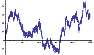
ListPlot[prices=Accumulate[sampleData]]

Chart 4


SSALGOTRADING AD

An Empirical Distribution

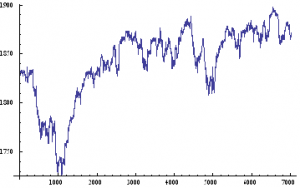
Lets take a look at a real price series, comprising 1 – minute bar data in the June ‘ 14 E – Mini futures contract.

Chart 5

As with our simulated price process, it is clear that the real price process for Emini futures is also non – stationary.

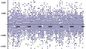
What about the returns process?

ListPlot[returnsES]

Chart 6

Notice the banding effect in returns, which results from having a fixed, minimum price move of $12 .50, rather than a continuous scale.

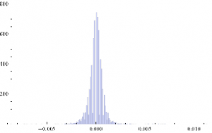
Histogram[returnsES]


Chart 7

Through[{Min,Max,Mean,Median,StandardDeviation,Skewness,Kurtosis}[returnsES]]

{-0.00867214,  0.0112353,  2.75501×10⁻⁶,   0.,   0.000780895,   0.35467,   26.2376}

The empirical returns distribution doesn’ t appear to be Gaussian – the distribution is much more peaked than a standard Normal distribution with the same mean and standard deviation. And the higher moments don’t fit the Normal model either – the empirical distribution has positive skew and a kurtosis that is almost 9x greater than a Gaussian distribution. The latter signifies what is often referred to as “fat tails”: the distribution has much greater weight in the tails than a standard Normal distribution, indicating a much greater likelihood of an extreme value than a Normal distribution would predict.

A Quantitative Analysis of Non-Stationarity: Two States

Non – stationarity arises when one or more of the moments of a distribution vary over time. Let’s take a look at how that can arise, and its effects.Suppose we have a Gaussian returns process for which the mean, or drift, or trend, fluctuates over time.

Let’s consider a simple example where the process drift is  μ1 and volatility σ1 for most of the time and then for some proportion of time k, we get addition drift  μ2 and volatility σ2.  In other words we have:

 Φ1=NormalDistribution[μ1,σ1]

 Through[{Mean,StandardDeviation,Skewness,Kurtosis}[Φ1]]

{μ1,   σ1,   0,   3}

 Φ2=NormalDistribution[μ2,σ2]

 Through[{Mean,StandardDeviation,Skewness,Kurtosis}[Φ2]]

{μ2,   σ2,   0,   3}

This simple model fits a scenario in which we suppose that the returns process spends most of its time in State 1, in which is Normally distributed with  drift is  μ1 and volatility σ1, and suffers from the occasional “shock” which propels the systems into a second State 2, in which its distribution is a combination of its original distribution and a new Gaussian distribution with different mean and volatility.

Let’ s suppose that we sample the combined process y =  Φ1 + k  Φ2.   What distribution would it have?  We can represent this is follows :

 y=TransformedDistribution[(x1+k x2),{x11,x22}]


Eqn2
 

 Through[{Mean,StandardDeviation,Skewness,Kurtosis}[y]]

Stationarity_52

 Plot[PDF[y,x]/.{μ10,μ20,σ1 1,σ2 2, k0.5},{x,-6,6},FillingAxis]

Chart 8

The result is just another Normal distribution. Depending on the incidence k, y will follow a Gaussian distribution whose mean and variance depend on the mean and variance of the two Normal distributions being mixed. The resulting distribution in State 2 may have higher or lower drift and volatility, but it is still Gaussian, with constant kurtosis of 3.

In other words, the system y will be non-stationary, because the first and second moments change over time, depending on what state it is in. But the form of the distribution is unchanged – it is still Gaussian. There are no fat-tails.

Non – Stationarity : Random States

In the above example the system moved between states in a known, predictable way. The “shocks” to the system were not really shocks, but transitions. But that’s not how financial markets behave: markets move from one state to another in an unpredictable way, with the arrival of news.

We can simulate this situation as follows. Using the former model as a starting point, lets now relax the assumption that the incidence of the second state, k, is a constant. Instead, let’ s assume that k is itself a random variable. In other words we are going to now assume that our system changes state in a random way. How does this alter the distribution?

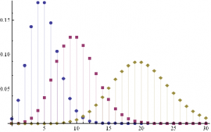
An appropriate model for λ might be a Poisson process, which is often used as a model for unpredictable, discrete events, ranging from bus arrivals to earthquakes.  PDFs of Poisson distributions with means  λ=5, 10 and 20 are shown in the chart below.  These represent probability distributions for processes that have mean  arrivals of 5, 10 or 20 events.

 DiscretePlot[Evaluate@Table[PDF[PoissonDistribution[λ],k],{λ,{5,10,20}}],{k,0,30},PlotRangeAll,PlotMarkersAutomatic]

Chart 9

Our new model now looks like this :

 y=TransformedDistribution[{x1+k*x2},{x1⎡Φ1,x2⎡Φ2,kPoissonDistribution[λ]}]

The first two moments of the distribution are as follows :

Through[{Mean,StandardDeviation}[y]]

Stationarity_60

As before, the mean and standard deviation of the distribution are going to vary, depending on the state of the system, and the mean arrival rate of shocks, . But what about kurtosis? Is it still constant?

Kurtosis[y]

Eqn1

Emphatically not!  The fourth moment of the distribution is now dependent on the drift in the second state, the volatilities of both states and the mean arrival rate of shocks, λ.

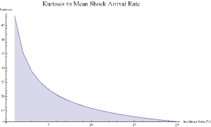
Let’ s look at a specific example.  Assume that in State 1 the process has volatility of 7.5 %, with zero drift, and that the shock distribution also has zero drift with volatility of 65 %. If the mean incidence rate of shocks λ = 10 %, the distribution kurtosis is close to that seen in the empirical distribution for the E-Mini.

 Kurtosis[y] /.{σ10.075,μ20,σ20.65,λ→0.1}

{35.3551}

More generally :

 ListLinePlot[Flatten[Kurtosis[y]/.Table[{σ10.075,μ20,σ20.65,λ→i/20},{i,1,20}]],PlotLabelStyle[“Kurtosis vs Mean Shock Arrival Rate”, FontSize18],AxesLabel->{“Incidence Rate (%)”, “Kurtosis”},FillingAxis, ImageSizeLarge]


Chart 10

Thus we can see how, even if the underlying returns distribution is Gaussian in form, the random arrival of news “shocks” to the system can induce non – stationarity in overall drift and volatility. It can also result in fat tails. More specifically, if the arrival of news is stochastic in nature, rather than deterministic, the process may exhibit far higher levels of kurtosis than in its original Gaussian state, in which the fourth moment was a constant level of 3.

Quantitative Analysis of a Jump Diffusion Process

Nobel – prize winning economist Robert Merton extended this basic concept to the realm of stochastic calculus.

In Merton’s jump diffusion model, the stock price follows the random process

∂St / St =μdt + σdWt+(J-1)dNt

The first two terms are familiar from the Black–Scholes model : drift rate μ, volatility σ, and random walk Wt (Wiener process).The last term represents the jumps :J is the jump size as a multiple of stock price, while Nt is the number of jump events that have occurred up to time t.is assumed to follow the Poisson process.

 PDF[PoissonDistribution[λt]]

where λ is the average frequency with which jumps occur.

The jump size J follows a log – normal distribution

 PDF[LogNormalDistribution[m, ν], s]

where m is the average jump size and v is the volatility of the jump size.

In the jump diffusion model, the stock price St follows the random process dSt/St=μ dt+σ dWt+(J-1) dN(t), which comprises, in order, drift, diffusive, and jump components. The jumps occur according to a Poisson distribution and their size follows a log-normal distribution. The model is characterized by the diffusive volatility σ, the average jump size J (expressed as a fraction of St), the frequency of jumps λ, and the volatility of jump size ν.

The Volatility Smile

The “implied volatility” corresponding to an option price is the value of the volatility parameter for which the Black-Scholes model gives the same price. A well-known phenomenon in market option prices is the “volatility smile”, in which the implied volatility increases for strike values away from the spot price. The jump diffusion model is a generalization of Black–Scholes in which the stock price has randomly occurring jumps in addition to the random walk behavior. One of the interesting properties of this model is that it displays the volatility smile effect. In this Demonstration, we explore the Black–Scholes implied volatility of option prices (equal for both put and call options) in the jump diffusion model. The implied volatility is modeled as a function of the ratio of option strike price to spot price.


The Mathematics of Scalping

NOTE:  if you are unable to see the Mathematica models below, you can download the free Wolfram CDF player and you may also need this plug-in.

You can also download the complete Mathematica CDF file here.

In this post I want to explore aspects of scalping, a type of strategy widely utilized by high frequency trading firms.

I will define a scalping strategy as one in which we seek to take small profits by posting limit orders on alternate side of the book. Scalping, as I define it, is a strategy rather like market making, except that we “lean” on one side of the book. So, at any given time, we may have a long bias and so look to enter with a limit buy order. If this is filled, we will then look to exit with a subsequent limit sell order, taking a profit of a few ticks. Conversely, we may enter with a limit sell order and look to exit with a limit buy order.
The strategy relies on two critical factors:

(i) the alpha signal which tells us from moment to moment whether we should prefer to be long or short
(ii) the execution strategy, or “trade expression”

In this article I want to focus on the latter, making the assumption that we have some kind of alpha generation model already in place (more about this in later posts).

There are several means that a trader can use to enter a position. The simplest approach, the one we will be considering here, is simply to place a single limit order at or just outside the inside bid/ask prices – so in other words we will be looking to buy on the bid and sell on the ask (and hoping to earn the bid-ask spread, at least).

SSALGOTRADING AD

One of the problems with this approach is that it is highly latency sensitive. Limit orders join the limit order book at the back of the queue and slowly works their way towards the front, as earlier orders get filled. Buy the time the market gets around to your limit buy order, there may be no more sellers at that price. In that case the market trades away, a higher bid comes in and supersedes your order, and you don’t get filled. Conversely, yours may be one of the last orders to get filled, after which the market trades down to a lower bid and your position is immediately under water.

This simplistic model explains why latency is such a concern – you want to get as near to the front of the queue as you can, as quickly as possible. You do this by minimizing the time it takes to issue and order and get it into the limit order book. That entails both hardware (co-located servers, fiber-optic connections) and software optimization and typically also involves the use of Immediate or Cancel (IOC) orders. The use of IOC orders by HFT firms to gain order priority is highly controversial and is seen as gaming the system by traditional investors, who may end up paying higher prices as a result.

Another approach is to layer limit orders at price points up and down the order book, establishing priority long before the market trades there. Order layering is a highly complex execution strategy that brings addition complications.

Let’s confine ourselves to considering the single limit order, the type of order available to any trader using a standard retail platform.

As I have explained, we are assuming here that, at any point in time, you know whether you prefer to be long or short, and therefore whether you want to place a bid or an offer. The issue is, at what price do you place your order, and what do you do about limiting your risk? In other words, we are discussing profit targets and stop losses, which, of course, are all about risk and return.

Risk and Return in Scalping

Lets start by considering risk. The biggest risk to a scalper is that, once filled, the market goes against his position until he is obliged to trigger his stop loss. If he sets his stop loss too tight, he may be forced to exit positions that are initially unprofitable, but which would have recovered and shown a profit if he had not exited. Conversely,  if he sets the stop loss too loose, the risk reward ratio is very low – a single loss-making trade could eradicate the profit from a large number of smaller, profitable trades.

Now lets think about reward. If the trader is too ambitious in setting his profit target he may never get to realize the gains his position is showing – the market could reverse, leaving him with a loss on a position that was, initially, profitable. Conversely, if he sets the target too tight, the trader may give up too much potential in a winning trade to overcome the effects of the occasional, large loss.

It’s clear that these are critical concerns for a scalper: indeed the trade exit rules are just as important, or even more important, than the entry rules. So how should he proceed?

Theoretical Framework for Scalping

Let’s make the rather heroic assumption that market returns are Normally distributed (in fact, we know from empirical research that they are not – but this is a starting point, at least). And let’s assume for the moment that our trader has been filled on a limit buy order and is looking to decide where to place his profit target and stop loss limit orders. Given a current price of the underlying security of X, the scalper is seeking to determine the profit target of p ticks and the stop loss level of q ticks that will determine the prices at which he should post his limit orders to exit the trade. We can translate these into returns, as follows:

to the upside: Ru = Ln[X+p] – Ln[X]

and to the downside: Rd = Ln[X-q] – Ln[X]

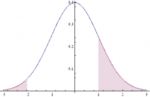
This situation is illustrated in the chart below.
Normal Distn Shaded

The profitable area is the shaded region on the RHS of the distribution. If the market trades at this price or higher, we will make money: p ticks, less trading fees and commissions, to be precise. Conversely we lose q ticks (plus commissions) if the market trades in the region shaded on the LHS of the distribution.

Under our assumptions, the probability of ending up in the RHS shaded region is:

probWin = 1 – NormalCDF(Ru, mu, sigma),

where mu and sigma are the mean and standard deviation of the distribution.

The probability of losing money, i.e. the shaded area in the LHS of the distribution, is given by:

probLoss = NormalCDF(Rd, mu, sigma),

where NormalCDF is the cumulative distribution function of the Gaussian distribution.

The expected profit from the trade is therefore:

Expected profit = p * probWin – q * probLoss

And the expected win rate, the proportion of profitable trades, is given by:

WinRate = probWin / (probWin + probLoss)

If we set a stretch profit target, then p will be large, and probWin, the shaded region on the RHS of the distribution, will be small, so our winRate will be low. Under this scenario we would have a low probability of a large gain. Conversely, if we set p to, say, 1 tick, and our stop loss q to, say, 20 ticks, the shaded region on the RHS will represent close to half of the probability density, while the shaded LHS will encompass only around 5%. Our win rate in that case would be of the order of 91%:

WinRate = 50% / (50% + 5%) = 91%

Under this scenario, we make frequent, small profits  and suffer the occasional large loss.

So the critical question is: how do we pick p and q, our profit target and stop loss?  Does it matter?  What should the decision depend on?

Modeling Scalping Strategies

We can begin to address these questions by noticing, as we have already seen, that there is a trade-off between the size of profit we are hoping to make, and the size of loss we are willing to tolerate, and the probability of that gain or loss arising.  Those probabilities in turn depend on the underlying probability distribution, assumed here to be Gaussian.

Now, the Normal or Gaussian distribution which determines the probabilities of winning or losing at different price levels has two parameters – the mean, mu, or drift of the returns process and sigma, its volatility.

Over short time intervals the effect of volatility outweigh any impact from drift by orders of magnitude.  The reason for this is simple:  volatility scales with the square root of time, while the drift scales linearly.  Over small time intervals, the drift becomes un-noticeably small, compared to the process volatility.  Hence we can assume that mu, the process mean is zero, without concern, and focus exclusively on sigma, the volatility.

What other factors do we need to consider?  Well there is a minimum price move, which might be 1 tick, and the dollar value of that tick, from which we can derive our upside and downside returns, Ru and Rd.  And, finally, we need to factor in commissions and exchange fees into our net trade P&L.

Here’s a simple formulation of the model, in which I am using the E-mini futures contract as an exemplar.

 WinRate[currentPrice_,annualVolatility_,BarSizeMins_, nTicksPT_, nTicksSL_,minMove_, tickValue_, costContract_]:=Module[{ nMinsPerDay, periodVolatility, tgtReturn, slReturn,tgtDollar, slDollar, probWin, probLoss, winRate, expWinDollar, expLossDollar, expProfit},
nMinsPerDay = 250*6.5*60;
periodVolatility = annualVolatility / Sqrt[nMinsPerDay/BarSizeMins];
tgtReturn=nTicksPT*minMove/currentPrice;tgtDollar = nTicksPT * tickValue;
slReturn = nTicksSL*minMove/currentPrice;
slDollar=nTicksSL*tickValue;
probWin=1-CDF[NormalDistribution[0, periodVolatility],tgtReturn];
probLoss=CDF[NormalDistribution[0, periodVolatility],slReturn];
winRate=probWin/(probWin+probLoss);
expWinDollar=tgtDollar*probWin;
expLossDollar=slDollar*probLoss;
expProfit=expWinDollar+expLossDollar-costContract;
{expProfit, winRate}]

For the ES contract we have a min price move of 0.25 and the tick value is $12.50.  Notice that we scale annual volatility to the size of the period we are trading (15 minute bars, in the following example).

Scenario Analysis

Let’s take a look at how the expected profit and win rate vary with the profit target and stop loss limits we set.  In the following interactive graphics, we can assess the impact of different levels of volatility on the outcome.

Expected Profit by Bar Size and Volatility

Expected Win Rate by Volatility

Notice to begin with that the win rate (and expected profit) are very far from being Normally distributed – not least because they change radically with volatility, which is itself time-varying.

For very low levels of volatility, around 5%, we appear to do best in terms of maximizing our expected P&L by setting a tight profit target of a couple of ticks, and a stop loss of around 10 ticks.  Our win rate is very high at these levels – around 90% or more.  In other words, at low levels of volatility, our aim should be to try to make a large number of small gains.

But as volatility increases to around 15%, it becomes evident that we need to increase our profit target, to around 10 or 11 ticks.  The distribution of the expected P&L suggests we have a couple of different strategy options: either we can set a larger stop loss, of around 30 ticks, or we can head in the other direction, and set a very low stop loss of perhaps just 1-2 ticks.  This later strategy is, in fact, the mirror image of our low-volatility strategy:  at higher levels of volatility, we are aiming to make occasional, large gains and we are willing to pay the price of sustaining repeated small stop-losses.  Our win rate, although still well above 50%, naturally declines.

As volatility rises still further, to 20% or 30%, or more, it becomes apparent that we really have no alternative but to aim for occasional large gains, by increasing our profit target and tightening stop loss limits.   Our win rate under this strategy scenario will be much lower – around 30% or less.

Non – Gaussian Model

Now let’s address the concern that asset returns are not typically distributed Normally. In particular, the empirical distribution of returns tends to have “fat tails”, i.e. the probability of an extreme event is much higher than in an equivalent Normal distribution.

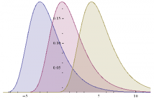
A widely used model for fat-tailed distributions in the Extreme Value Distribution. This has pdf:

PDF[ExtremeValueDistribution[,],x]

 EVD

Plot[Evaluate@Table[PDF[ExtremeValueDistribution[,2],x],{,{-3,0,4}}],{x,-8,12},FillingAxis]
EVD pdf

Mean[ExtremeValueDistribution[,]]

+EulerGamma

Variance[ExtremeValueDistribution[,]]

EVD Variance

In order to set the parameters of the EVD, we need to arrange them so that the mean and variance match those of the equivalent Gaussian distribution with mean = 0 and standard deviation . hence:

EVD params

The code for a version of the model using the GED is given as follows

WinRateExtreme[currentPrice_,annualVolatility_,BarSizeMins_, nTicksPT_, nTicksSL_,minMove_, tickValue_, costContract_]:=Module[{ nMinsPerDay, periodVolatility, alpha, beta,tgtReturn, slReturn,tgtDollar, slDollar, probWin, probLoss, winRate, expWinDollar, expLossDollar, expProfit},
nMinsPerDay = 250*6.5*60;
periodVolatility = annualVolatility / Sqrt[nMinsPerDay/BarSizeMins];
beta = Sqrt[6]*periodVolatility / Pi;
alpha=-EulerGamma*beta;
tgtReturn=nTicksPT*minMove/currentPrice;tgtDollar = nTicksPT * tickValue;
slReturn = nTicksSL*minMove/currentPrice;
slDollar=nTicksSL*tickValue;
probWin=1-CDF[ExtremeValueDistribution[alpha, beta],tgtReturn];
probLoss=CDF[ExtremeValueDistribution[alpha, beta],slReturn];
winRate=probWin/(probWin+probLoss);
expWinDollar=tgtDollar*probWin;
expLossDollar=slDollar*probLoss;
expProfit=expWinDollar+expLossDollar-costContract;
{expProfit, winRate}]

WinRateExtreme[1900,0.05,15,2,30,0.25,12.50,3][[2]]

0.21759

We can now produce the same plots for the EVD version of the model that we plotted for the Gaussian versions :

Expected Profit by Bar Size and Volatility – Extreme Value Distribution

Expected Win Rate by Volatility – Extreme Value Distribution

Next we compare the Gaussian and EVD versions of the model, to gain an understanding of how the differing assumptions impact the expected Win Rate.

Expected Win Rate by Stop Loss and Profit Target

As you can see, for moderate levels of volatility, up to around 18 % annually, the expected Win Rate is actually higher if we assume an Extreme Value distribution of returns, rather than a Normal distribution.If we use a Normal distribution we will actually underestimate the Win Rate, if the actual return distribution is closer to Extreme Value.In other words, the assumption of a Gaussian distribution for returns is actually conservative.

Now, on the other hand, it is also the case that at higher levels of volatility the assumption of Normality will tend to over – estimate the expected Win Rate, if returns actually follow an extreme value distribution. But, as indicated before, for high levels of volatility we need to consider amending the scalping strategy very substantially. Either we need to reverse it, setting larger Profit Targets and tighter Stops, or we need to stop trading altogether, until volatility declines to normal levels.Many scalpers would prefer the second option, as the first alternative doesn’t strike them as being close enough to scalping to justify the name.If you take that approach, i.e.stop trying to scalp in periods when volatility is elevated, then the differences in estimated Win Rate resulting from alternative assumptions of return distribution are irrelevant.

If you only try to scalp when volatility is under, say, 20 % and you use a Gaussian distribution in your scalping model, you will only ever typically under – estimate your actual expected Win Rate.In other words, the assumption of Normality helps, not hurts, your strategy, by being conservative in its estimate of the expected Win Rate.

If, in the alternative, you want to trade the strategy regardless of the level of volatility, then by all means use something like an Extreme Value distribution in your model, as I have done here.That changes the estimates of expected Win Rate that the model produces, but it in no way changes the structure of the model, or invalidates it.It’ s just a different, arguably more realistic set of assumptions pertaining to situations of elevated volatility.

Monte-Carlo Simulation Analysis

Let’ s move on to do some simulation analysis so we can get an understanding of the distribution of the expected Win Rate and Avg Trade PL for our two alternative models. We begin by coding a generator that produces a sample of 1,000 trades and calculates the Avg Trade PL and Win Rate.

Gaussian Model

GenWinRate[currentPrice_,annualVolatility_,BarSizeMins_, nTicksPT_, nTicksSL_,minMove_, tickValue_, costContract_]:=Module[{ nMinsPerDay, periodVolatility, randObs, tgtReturn, slReturn,tgtDollar, slDollar, nWins,nLosses, perTradePL, probWin, probLoss, winRate, expWinDollar, expLossDollar, expProfit},
nMinsPerDay = 250*6.5*60;
periodVolatility = annualVolatility / Sqrt[nMinsPerDay/BarSizeMins];
tgtReturn=nTicksPT*minMove/currentPrice;tgtDollar = nTicksPT * tickValue;
slReturn = nTicksSL*minMove/currentPrice;
slDollar=nTicksSL*tickValue;
randObs=RandomVariate[NormalDistribution[0,periodVolatility],10^3];
nWins=Count[randObs,x_/;x>=tgtReturn];
nLosses=Count[randObs,x_/;xslReturn];
winRate=nWins/(nWins+nLosses)//N;
perTradePL=(nWins*tgtDollar+nLosses*slDollar)/(nWins+nLosses);{perTradePL,winRate}]

GenWinRate[1900,0.1,15,1,-24,0.25,12.50,3]

{7.69231,0.984615}

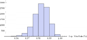
Now we can generate a random sample of 10, 000 simulation runs and plot a histogram of the Win Rates, using, for example, ES on 5-min bars, with a PT of 2 ticks and SL of – 20 ticks, assuming annual volatility of 15 %.

Histogram[Table[GenWinRate[1900,0.15,5,2,-20,0.25,12.50,3][[2]],{i,10000}],10,AxesLabel{“Exp. Win Rate (%)”}]
WinRateHist

Histogram[Table[GenWinRate[1900,0.15,5,2,-20,0.25,12.50,3][[1]],{i,10000}],10,AxesLabel{“Exp. PL/Trade ($)”}]
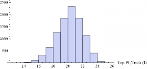
PLHist

Extreme Value Distribution Model

Next we can do the same for the Extreme Value Distribution version of the model.

GenWinRateExtreme[currentPrice_,annualVolatility_,BarSizeMins_, nTicksPT_, nTicksSL_,minMove_, tickValue_, costContract_]:=Module[{ nMinsPerDay, periodVolatility, randObs, tgtReturn, slReturn,tgtDollar, slDollar, alpha, beta,nWins,nLosses, perTradePL, probWin, probLoss, winRate, expWinDollar, expLossDollar, expProfit},
nMinsPerDay = 250*6.5*60;
periodVolatility = annualVolatility / Sqrt[nMinsPerDay/BarSizeMins];
beta = Sqrt[6]*periodVolatility / Pi;
alpha=-EulerGamma*beta;
tgtReturn=nTicksPT*minMove/currentPrice;tgtDollar = nTicksPT * tickValue;
slReturn = nTicksSL*minMove/currentPrice;
slDollar=nTicksSL*tickValue;
randObs=RandomVariate[ExtremeValueDistribution[alpha, beta],10^3];
nWins=Count[randObs,x_/;x>=tgtReturn];
nLosses=Count[randObs,x_/;xslReturn];
winRate=nWins/(nWins+nLosses)//N;
perTradePL=(nWins*tgtDollar+nLosses*slDollar)/(nWins+nLosses);{perTradePL,winRate}]

Histogram[Table[GenWinRateExtreme[1900,0.15,5,2,-10,0.25,12.50,3][[2]],{i,10000}],10,AxesLabel{“Exp. Win Rate (%)”}]
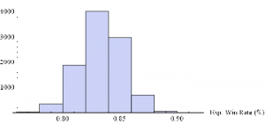
WinRateEVDHist

Histogram[Table[GenWinRateExtreme[1900,0.15,5,2,-10,0.25,12.50,3][[1]],{i,10000}],10,AxesLabel{“Exp. PL/Trade ($)”}]
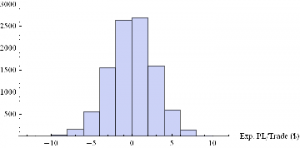
PLEVDHist


Conclusions

The key conclusions from this analysis are:

  1. Scalping is essentially a volatility trade
  2. The setting of optimal profit targets are stop loss limits depend critically on the volatility of the underlying, and needs to be handled dynamically, depending on current levels of market volatility
  3. At low levels of volatility we should set tight profit targets and wide stop loss limits, looking to make a high percentage of small gains, of perhaps 2-3 ticks.
  4. As volatility rises, we need to reverse that position, setting more ambitious profit targets and tight stops, aiming for the occasional big win.
 

How to Spot a Fake

One of the issues that comes up regularly is how, as an investor or other interested party, one can protect oneself from unscrupulous scam artists posing as professional traders or money managers. This is a particular problem on web sites featuring trader forums, where individuals with unverified track records claiming stellar trading histories use their purported trading “prowess” to try to impress and intimidate other participants, usually impressionable newbies. The purpose of this post is to provide some guidance to help investors, traders and other fellow travelers sort the wheat from the chaff. We’ll be doing some forensic analysis on the track record for a strategy in NG futures that one such character recently posted in one of these forums, as a classic example of the kind of fakery I am describing.

One thing you should understand about scam artists operating on forums, is that they don’t work alone: usually they have a bunch of groupies who will shill for them at every opportunity and who will try to shout down any investigative questioning. Don’t be deterred. These know-it-alls are usually just ignorant dupes, who understand no more about trading than the scam artist. They may just as easily be fellow-scam artists themselves.

THE FIRST BIG RED FLAG: UNWILLINGNESS TO PRODUCE A TRACK RECORD
Anyone claiming to be a CTA or professional money manager (or whose shills claim he is one) has to have a track record that is freely available in the public domain. So how does a scam artist overcome a challenge to produce it? He will claim that he “can’t advertise”, or make some other, similar excuse. Don’t accept that at face value. Ask him to PM it to you. If he won’t, there’s already a high probability he’s a con artist.
THE SECOND BIG RED FLAG: CURVE FITTING
Let’s say our suspect meets the challenge and produces a track record. Ideally this will be an audited P&L statement, but let’s assume for the purposes of this discussion that he produces something along the lines of the Performance Reports produced by a product like Tradestation or MultiCharts, i.e. we are dealing with a simulated back-test.

If your suspect produces a back-test, you can be pretty sure it’s going to look good – otherwise he wouldn’t produce it. The task now is to dig into those reports to spot the red flags that give clues as to whether it might be fake.
Now of course any trading system is going to make assumptions – about fill rates, slippage, commissions, capacity etc. All that is fine, as long as the assumptions are clearly stated. You might want to challenge any or all of the assumptions, and the trader may disagree with you about some or all of them. That’s perfectly ok – it’s an honest, open discussion about a set of investment assumptions that have been revealed at the outset.

But here is what is NOT ok: any opacity about which data was used to build the trading model and which data was used to test it. The former, the in-sample (IS) data set, used to construct the model, must be entirely separate and distinct from the out-of-sample (OOS) data set. It is trivially easy using a tool like Tradestation to produce a trading system that shows stellar results in-sample, but which will immediately crash and burn when it is used in live trading. This is known as curve-fitting. And it’s by far the most common method by which scam artists try to dupe investors.

In order to demonstrate the robustness of the system prior to risking real money, a genuine trader will test his system OOS and show you the results. What you are looking for ideally is congruity between the IS and OOS results. Now by congruity, I don’t mean that they should be identical. Far from it – markets evolve and strategy performance will vary over time. But what you are hoping is that the key performance metrics in the OOS and IS periods, such as annual returns, Sharpe ratio, PNL per contract, profit ratio and win rate, will be comparable. At the very least, you would like to be able to identify some portion of the IS data set for which the strategy performance characteristics are similar to those in the OOS period.

Any – I mean ANY – ambiguity or lack of clarity about which data was used to build the model and which was used for OOS testing is a HUGE red flag. Chances are, your scam artist is already trying to fudge the issue that he curve-fitted the system.
This was the case in the recent forum post we are using as a test case. The trader made no attempt whatsoever to clarify which data was used for model development and which for testing. Immediately, I was suspicious and began looking for other evidence of curve fitting. It didn’t take me long to find it.

THE THIRD BIG RED FLAG: THE EQUITY CURVE
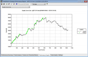
The first item I turned to in the performance reports was the equity curve and I immediately spotted two rather large clues that I was dealing with a fake.

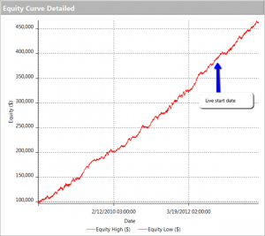
The first clue was the large sign on the chart labelled “live start date”. What does this mean? This is a back-test, so all of the results are theoretical, including those after the supposed “live start date” sometime in 2013. What the faker is trying to do is imply the part of the equity curve shown after that date indicate actual performance results. He doesn’t actually claim this, so he has plausible deniability if you call him on it (“I said it was just a back test”). But he hopes that you won’t, and that, by default, you’ll accept these results are real. But they aren’t.

The second clue of fakery is much more important: the equity curve itself. When someone shows you and equity curve like the one reported by this trader, rising in a straight line from the lower left to upper right quadrants, you can be 99% confident that you are dealing with a fake.
You see, in finance there are almost never any straight lines. They are as rare as unicorns. Especially when it comes to strategy performance. They only time you will EVER see an equity curve like this is when you are looking at the equity curve of (i) a high frequency market making trading system or (ii) a fake, produced by curve fitting a strategy to the ENTIRE data set.
And this strategy was not high frequency – as we shall see, it operated on 15 minute bars, holding positions overnight.

EC Chart

THE FOURTH BIG RED FLAG: GOD’s EQUITY CURVE
I said that straight line equity curve were extremely rare. In fact, even God’s equity curve isn’t often a straight line. What does that mean?

Suppose you had a strategy that could predict with 100% accuracy whether the market would go up or down over the next bar (whether you are using daily bars, or 15 minute bars, as in our example). The system would buy (or hold) when the market was forecast to rise, and sell when the market was predicted to fall. What would the performance of such a perfect system look like? Pretty stellar, obviously. And most people would guess that the system’s equity curve would be a straight line, or maybe even exponential in shape. In fact that’s typically not the case. God’s equity curve will be sloped and kinked, just like any other equity curve. And if your suspect’s equity curve is real, it should show some commonality with God’s equity curve, by which I mean it should show changes in slope and level that reflect those seen in the perfect equity curve.

What does God’s Equity Curve look like in NG futures?

Gods EC

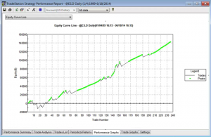
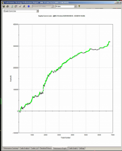
As you can see it’s not straight. In fact it’s concave. So a REAL equity curve should have similar characteristics, like this one, for example:

NG EC

As you can see, the equity curve of the real trading system track’s God’s Equity Curve, albeit at a much lower level. It’s concave, with an upswing during the final few months of trading, just like God’s. That’s a good sign that the strategy back-test is very likely genuine (which it is – I produced it).

Why is Gods’ Equity Curve the shape it is? The answer will vary from market to market. In the case of NG, the suggestion is that the market is becoming more efficient: simple trading strategies based on technical indicators work less well than they did five years ago. We have seen something very similar in F/X markets. During the 1970’s and 1980’s when Soros was active in the field, simple strategies like moving average crossovers made great returns, but these entirely dissipated in the 1990’s, with the advent of widely available computing power.

THE FIFTH BIG RED FLAG: THE SHILL SHOUTDOWN
When I posted my analysis, which clearly indicated fakery by this well known forum participant, I was immediately flamed by one of his supporters who shouted something to the effect that (i) everyone knows that the downward slope of God’s Equity Curve was caused by volatility and (ii) the star trader, unlike God, or me, knows about position sizing.

This attempt at misdirection in the face of awkward facts is a classic sign of fakery. What distinguishes the shill post is:

(i) Immediacy – clearly no attempt has been made to evaluate the argument or analysis. The shill simply attempts to drown out the critic with a lot of noise, as quickly as possible.

(ii) Plausibility – shills will throw around terms that lend plausibility to their objection, but which after a moment’s reflection are entirely irrelevant or, as in this case, detrimental to their own cause.

(iii) Invective – the more intemperate the post, the more likely the shill is simply trying to provide cover for the faker.

So let’s take a moment to dispose of the plausible sounding objections posted by the shill in this example.
I am going to take it as read that everyone understands that trading profitability is positively correlated with volatility. There is a huge amount of empirical research supporting that finding, but to keep it simple we can appeal to one of the cornerstones of modern finance: risk and return. The higher the volatility, i.e. the greater the risk, the greater the return traders and investors in the markets will require on their capital. This is a principle of modern financial theory that even a graduate of the Scranton college of fine art should be expected to appreciate.
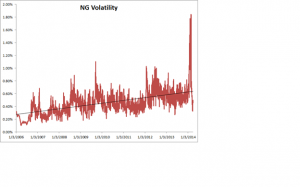
So what’s the story with NG volatility? You can see the time series of NG volatility in the chart below. One feature stands out above all others: the upward slope of the curve. NG volatility has RISEN over the sample period from 2008 to 2014. Consequently, returns from trading NG futures should also have RISEN rather than fallen. One thing we can say for sure, whatever caused the concave shape in God’s Equity Curve in NG futures, it was NOT volatility!

NG Volatility

Turning to the shill’s next, plausible sounding, but dubious “explanation”, position sizing: this really is completely irrelevant. Because, as we shall see from an examination of the performance report, the track record was created by trading a constant one-lot! So this was just an attempt to sound “sophisticated” by someone trying to misdirect the reader away from the increasingly obvious evidence of fakery.

THE SIXTH BIG RED FLAG: LOW DRAWDOWNS AND OVERNIGHT GAP RISK
One of the highly unusual features of our faker’s equity curve is it’s exceptional smoothness. Low volatility in the equity curve is, in and of itself, an indicator the track record results from curve fitting. But we can get even more insight by digging into the performance report, shown below.

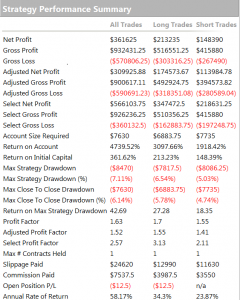
Perf 1
Perf 2

As you can see from the second page of the report, the strategy holds positions for an average of 57 15-minute bars, equivalent to slightly over 14 hours. So this is a low frequency strategy that takes overnight risk. Now, as any trader will know, overnight gap risk in a product like NG can be very significant and likely to be produce much larger drawdowns over a 5 year period than the $8,470 reported here.

The only other possible explanation is that the strategy is traded continuously through both day and night sessions. But this is not only itself improbable, it gives rise to another implausibility: liquidity in the overnight session is so poor that the strategy is unlikely to be able to trade more than 1-2 contracts, at most. This would be of little value to a CTA, or its customers, whatever the star trader’s protestations that his “clients are happy”.

There is no plausible way to resolve the disconnection between the low drawdown, overnight gap risk and market illiquidity. The most plausible explanation: the back-test is a curve fitting exercise.

THE SEVENTH AN FINAL BIG RED FLAG: INCONSISTENCY BETWEEN PERFORMANCE METRICS
As any experienced strategy developer knows, you can get some of the things you want, but you can never achieve all of them. Amongst the desirable features to be maximized are
• Profit factor
• Average PNL per contract
• Percentage win rate

There is a trade-off between the features. A high PNL per contract typically means you are trading less frequently, with longer hold periods, and consequently the percentage win rate tends to be lower. Alternatively, you can increase the win rate, at the cost of lowering the average PNL per contract and/or the profit factor. And so on.

This strategy purports to have it all: a high average PNL per contract resulting from low frequency trading, coupled with good percentage win rate of over 50% and profit factor. A win rate of much over 40% is highly unusual for a momentum strategy entering and exiting with market or stop orders – and its almost inconceivable for a strategy with a PNL per contract and profit factor as large as suggested here.

CONCLUSION
This back-test fails the sniff test on so many levels, I would rate the chance of it being real as less than 1 in 1000.
The final, conclusive proof of fakery is that the “star trader” responsible for producing the report was unable and/or unwilling to attempt to answer even a single one of the criticisms.

So, be warned. If you see forum members banding about track records like this one, you can be sure that they and their strategies are likely to be fake, and not to be trusted.

Metaprogramming and the Future of the Wolfram Language

The Accelerating Pace of Functionality Development

With all the marvelous new functionality that we have come to expect with each release, it is sometimes challenging to maintain a grasp on what the Wolfram language encompasses currently, let alone imagine what it might look like in another ten years. Indeed, the pace of development appears to be accelerating, rather than slowing down. However, I predict that the “problem” is soon about to get much, much worse. What I foresee is a step change in the pace of development of the Wolfram Language that will produce in days and weeks, or perhaps even hours and minutes, functionality might currently take months or years to develop. So obvious and clear cut is this development that I have hesitated to write about it, concerned that I am simply stating something that is blindingly obvious to everyone. But I have yet to see it even hinted at by others, including Wolfram. I find this surprising, because it will revolutionize the way in which not only the Wolfram language is developed in future, but in all likelihood programming and language development in general.

Wolfram Language as an Object

The key to this paradigm shift lies in the following unremarkable-looking WL function WolframLanguageData[], which gives a list of all Wolfram Language symbols and their properties. So, for example, we have:

WolframLanguageData[“SampleEntities”]


This means we can treat WL language constructs as objects, query their properties and apply functions to them, such as, for example:

WolframLanguageData[“Cos”, “RelationshipCommunityGraph”]

In other words, the WL gives us the ability to traverse the entirety of the WL itself, combining WL objects into expressions, or programs.

Metaprogramming & Genetic Programming

This process is one definition of the term “Metaprogramming”. What I am suggesting is that in future, much of the heavy lifting will be carried out, not by developers, but by WL programs designed to produce code by metaprogramming. If successful, such an approach could streamline and accelerate the development process, speeding it up many times and, eventually, opening up areas of development that are currently beyond our imagination (and, possibly, our comprehension). So how does one build a metaprogramming system? This is where I should hand off to a computer scientist (and will happily do so as soon as one steps forward to take up the discussion). But here is a simple outline of one approach.

The principal tool one might use for such a task is genetic programming:

WikipediaData[“Genetic Programming”]


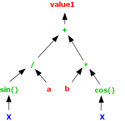
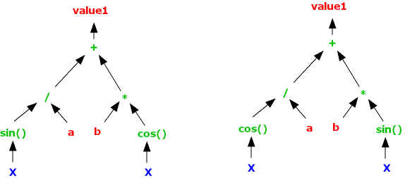
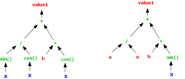
Actually, one can take issue with this explanation on several fronts, in particular the suggestion that GP is used primarily as a means of generating a computer program for performing a predefined task. That may certainly be the case, but need not be. Leaving that aside, the idea in simple terms is that we write a program that traverses the WL structure in some way, splicing together language objects to create a WL program that “does something”. That “something” may be a predefined task and indeed this would be a great place to start: to write a GP Metaprogramming system that creates programs that replicate the functionality of existing WL functions. Most of the generated programs would likely be uninteresting, slower versions of existing functions; but it is conceivable, I suppose, that some of the results might be of academic interest, or indicate a potentially faster computation method, perhaps. However, the point of the exercise is to get started on the Metaprogramming project, with a simple(ish) task with very clear, pre-defined goals and producing results that are easily tested. In this case the “objective function” is a comparison of results produced by the inbuilt WL functions vs the GP-generated functions, across some selected domain for the inputs. I glossed over the question of exactly how one “traverses the WL structure” for good reason: I feel quite sure that there must have been tremendous advances in the theory of how to do this in the last 50 years. But just to get the ball rolling, one could, for instance, operate a dual search, with a local search evaluating all of the functions closely connected to the (randomly chosen) starting function (WL object, while a second “long distance” search routine jumps randomly to a group of functions some specified number of steps away from the starting function. [At this point I envisage the computer scientists rolling their eyes and muttering “doesn’t this idiot know about the {fill in the blank} theorem about efficient domain search algorithms?”]. Anyway, to continue.

The Wolfram One-Liner Competition as an Exercise in Metaprogramming

The initial exercise described above is about the mechanics of the process rather that the outcome. The second stage is much more challenging, as the goal is to develop new functionality, rather than simply to replicate what already exists. It would entail defining a much more complex objective function, as well as perhaps some constraints on program size, the number and types of WL objects used, etc. An interesting exercise, for example, would be to try to develop a metaprogramming system capable of winning the Wolfram One-Liner contest. Here, one might characterize the objective function as “something interesting and surprising”, and we would impose a tight constraint on the length of programs generated by the metaprogramming system to a single line of code. What is “interesting and surprising”? To be defined – that’s a central part of the challenge. But, in principle, I suppose one might try to train a neural network to classify whether or not a result is “interesting” based on the results of prior one-liner competitions.

From there, it’s on to the hard stuff: designing metaprogramming systems to produce WL programs of arbitrary length and complexity to do “interesting stuff” in a specific domain. That “interesting stuff” could be a more efficient approximation for a certain type of computation, a new algorithm for detecting certain patterns, or coming up with some completely novel formula or computational concept.

Conclusion:  the Challenge of Metaprogramming

Obviously one faces huge challenges with this undertaking; but the potential rewards are enormous in terms of accelerating the pace of language development and discovery. It is a fascinating area for R&D, one that the WL is ideally situated to exploit. Indeed, I would be mightily surprised to learn that there is not already a team engaged on just such research at Wolfram. If so, perhaps one of them could comment here?