In his latest book (Algorithmic Trading: Winning Strategies and their Rationale, Wiley, 2013) Ernie Chan does an excellent job of setting out the procedures for developing statistical arbitrage strategies using cointegration. In such mean-reverting strategies, long positions are taken in under-performing stocks and short positions in stocks that have recently outperformed.
I will leave a detailed description of the procedure to Ernie (see pp 47 – 60), which in essence involves:
(i) estimating a cointegrating relationship between two or more stocks, using the Johansen procedure
(ii) computing the half-life of mean reversion of the cointegrated process, based on an Ornstein-Uhlenbeck representation, using this as a basis for deciding the amount of recent historical data to be used for estimation in (iii)
(iii) Taking a position proportionate to the Z-score of the market value of the cointegrated portfolio (subtracting the recent mean and dividing by the recent standard deviation, where “recent” is defined with reference to the half-life of mean reversion)
Countless researchers have followed this well worn track, many of them reporting excellent results. In this post I would like to discuss a few of many considerations in the procedure and variations in its implementation. We will follow Ernie’s example, using daily data for the EWF-EWG-ITG triplet of ETFs from April 2006 – April 2012. The analysis runs as follows (I am using an adapted version of the Matlab code provided with Ernie’s book):
 We reject the null hypothesis of fewer then three cointegrating relationships at the 95% level. The eigenvalues and eigenvectors are as follows:
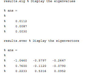 The eignevectors are sorted by the size of their eigenvalues, so we pick the first of them, which is expected to have the shortest half-life of mean reversion, and create a portfolio based on the eigenvector weights (-1.046, 0.76, 0.2233). From there, it requires a simple linear regression to estimate the half-life of mean reversion:
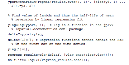 From which we estimate the half-life of mean reversion to be 23 days. This estimate gets used during the final, stage 3, of the process, when we choose a look-back period for estimating the running mean and standard deviation of the cointegrated portfolio. The position in each stock (numUnits) is sized according to the standardized deviation from the mean (i.e. the greater the deviation the larger the allocation).
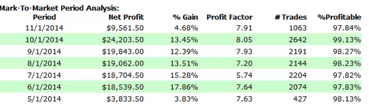
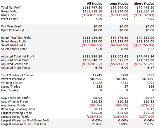
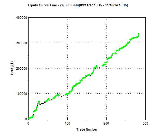
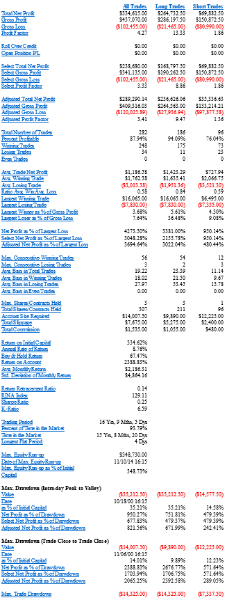
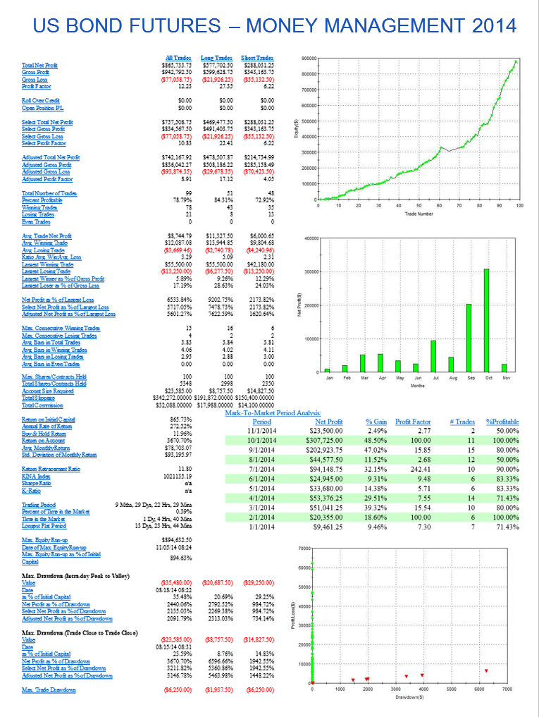
 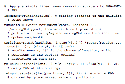 The results appear very promising, with an annual APR of 12.6% and Sharpe ratio of 1.4:
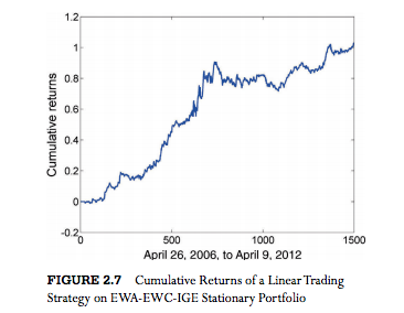
Ernie is at pains to point out that, in this and other examples in the book, he pays no attention to transaction costs, nor to the out-of-sample performance of the strategies he evaluates, which is fair enough.
The great majority of the academic studies that examine the cointegration approach to statistical arbitrage for a variety of investment universes do take account of transaction costs. For the most part such studies report very impressive returns and Sharpe ratios that frequently exceed 3. Furthermore, unlike Ernie’s example which is entirely in-sample, these studies typically report consistent out-of-sample performance results also.
But the single, most common failing of such studies is that they fail to consider the per share performance of the strategy. If the net P&L per share is less than the average bid-offer spread of the securities in the investment portfolio, the theoretical performance of the strategy is unlikely to survive the transition to implementation. It is not at all hard to achieve a theoretical Sharpe ratio of 3 or higher, if you are prepared to ignore the fact that the net P&L per share is lower than the average bid-offer spread. In practice, however, any such profits are likely to be whittled away to zero in trading frictions – the costs incurred in entering, adjusting and exiting positions across multiple symbols in the portfolio.
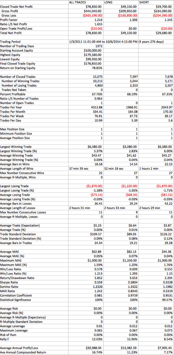
Put another way, you would want to see a P&L per share of at least 1c, after transaction costs, before contemplating implementation of the strategy. In the case of the EWA-EWC-IGC portfolio the P&L per share is around 3.5 cents. Even after allowing, say, commissions of 0.5 cents per share and a bid-offer spread of 1c per share on both entry and exit, there remains a profit of around 2 cents per share – more than enough to meet this threshold test.
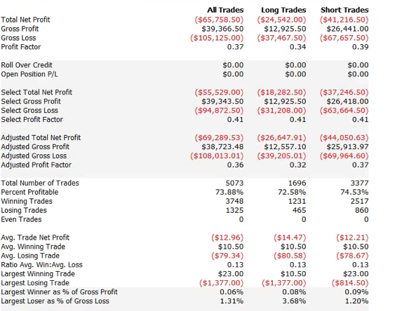
Let’s address the second concern regarding out-of-sample testing. We’ll introduce a parameter to allow us to select the number of in-sample days, re-estimate the model parameters using only the in-sample data, and test the performance out of sample. With a in-sample size of 1,000 days, for instance, we find that we can no longer reject the null hypothesis of fewer than 3 cointegrating relationships and the weights for the best linear portfolio differ significantly from those estimated using the entire data set.
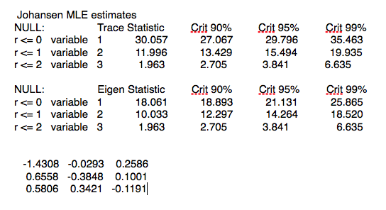
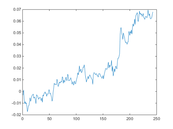
Repeating the regression analysis using the eigenvector weights of the maximum eigenvalue vector (-1.4308, 0.6558, 0.5806), we now estimate the half-life to be only 14 days. The out-of-sample APR of the strategy over the remaining 500 days drops to around 5.15%, with a considerably less impressive Sharpe ratio of only 1.09.
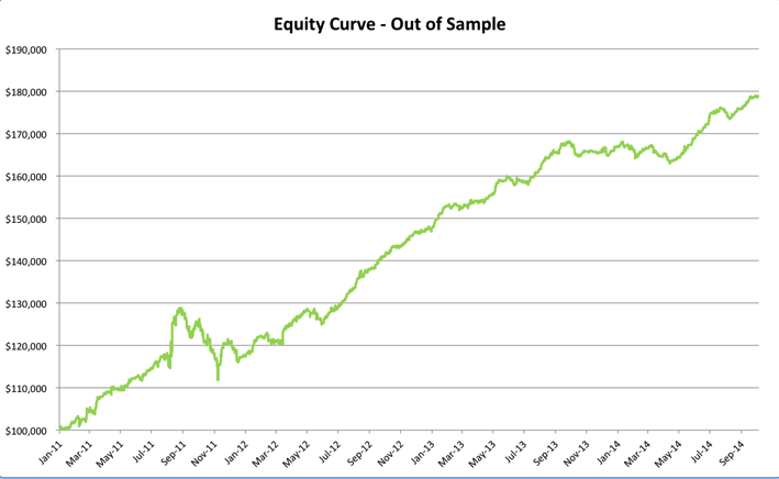
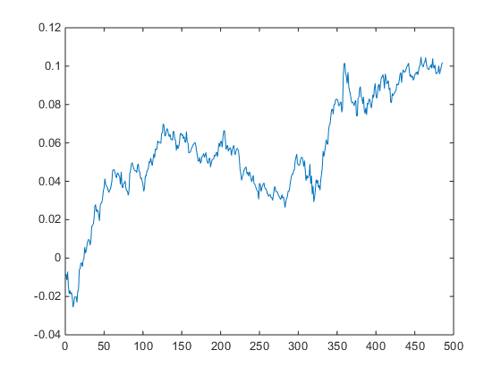 Out-of-sample cumulative returns
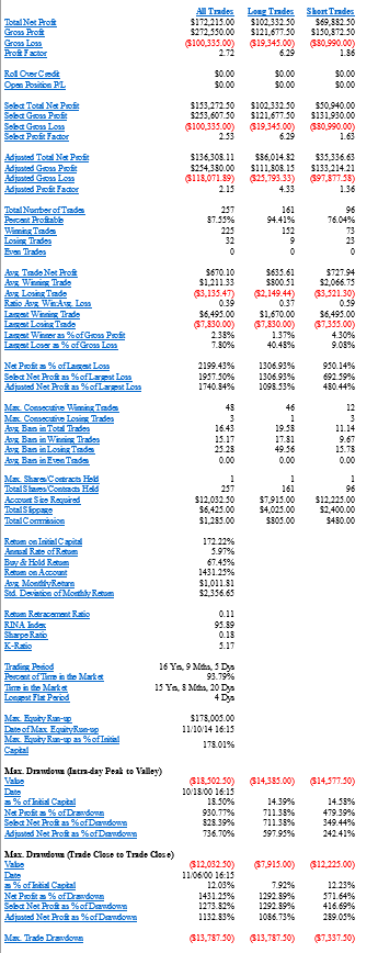
One way to improve the strategy performance is to relax the assumption of strict proportionality between the portfolio holdings and the standardized deviation in the market value of the cointegrated portfolio. Instead, we now require the standardized deviation of the portfolio market value to exceed some chosen threshold level before we open a position (and we close any open positions when the deviation falls below the threshold). If we choose a threshold level of 1, (i.e. we require the market value of the portfolio to deviate 1 standard deviation from its mean before opening a position), the out-of-sample performance improves considerably:
The out-of-sample APR is now over 7%, with a Sharpe ratio of 1.45.
The strict proportionality requirement, while logical, is rather unusual: in practice, it is much more common to apply a threshold, as I have done here. This addresses the need to ensure an adequate P&L per share, which will typically increase with higher thresholds. A countervailing concern, however, is that as the threshold is increased the number of trades will decline, making the results less reliable statistically. Balancing the two considerations, a threshold of around 1-2 standard deviations is a popular and sensible choice.
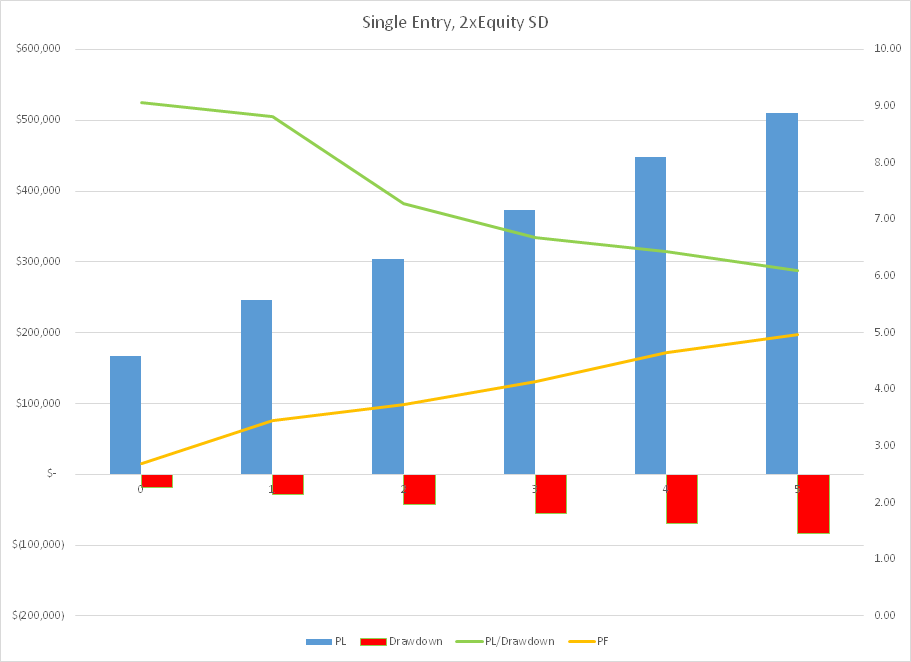
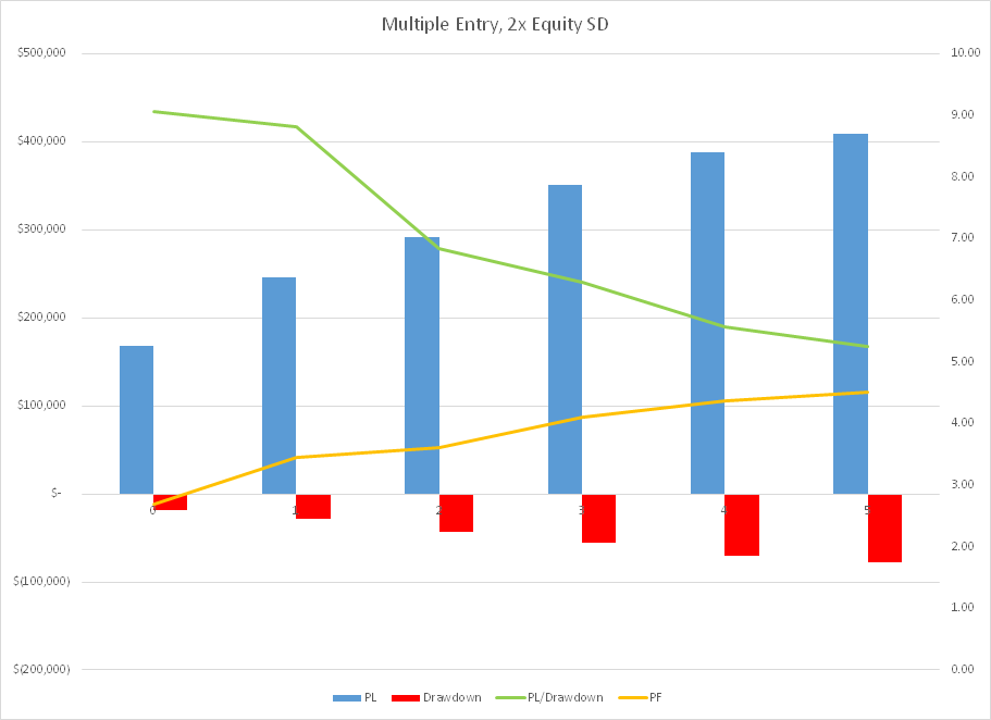
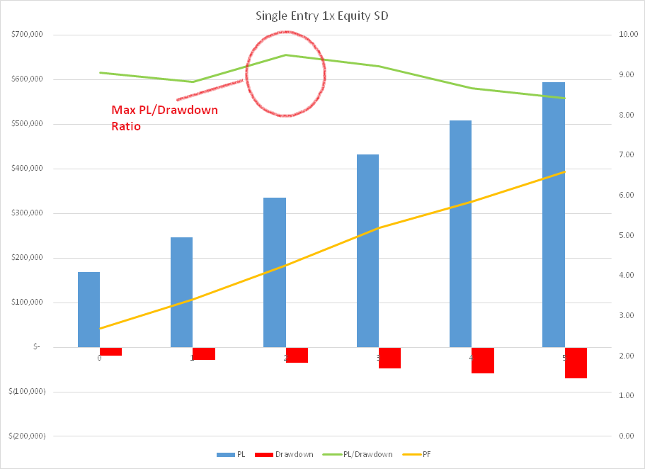
Of course, introducing thresholds opens up a new set of possibilities: just because you decide to enter based on a 2x SD trigger level doesn’t mean that you have to exit a position at the same level. You might consider the outcome of entering at 2x SD, while exiting at 1x SD, 0x SD, or even -2x SD. The possible nuances are endless.
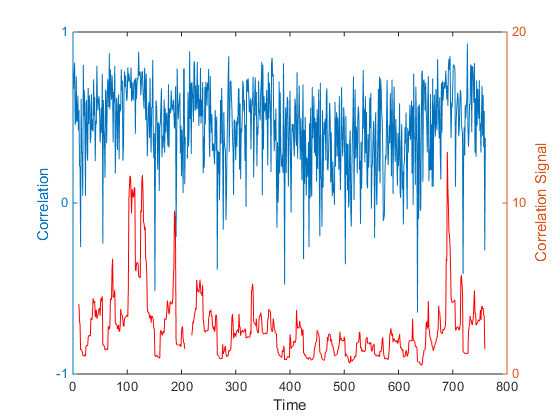
Unfortunately, the inconsistency in the estimates of the cointegrating relationships over different data samples is very common. In fact, from my own research, it is often the case that cointegrating relationships break down entirely out-of-sample, just as do correlations. A recent study by Matthew Clegg of over 860,000 pairs confirms this finding (On the Persistence of Cointegration in Pais Trading, 2014) that cointegration is not a persistent property.
I shall examine one approach to addressing the shortcomings of the cointegration methodology in a future post.
Matlab code (adapted from Ernie Chan’s book):
Continue reading “Developing Statistical Arbitrage Strategies Using Cointegration”