Equities Archives - Page 2 of 3 - QUANTITATIVE RESEARCH AND TRADING

May 26, 2020

Finding Alpha in 2018

Given the current macro-economic environment, where should investors focus their search for sources of alpha in the year ahead? By asking enough economists or investment managers you will find as many different opinions on the subject as would care to, no doubt many of them conflicting. These are some thoughts on the subject from my perspective, as a quantitative hedge fund manager.

Global Market Performance in 2017

Let’s begin by reviewing some of the best and worst performing assets of 2017 (I am going to exclude cryptocurrencies from the ensuing discussion). Broadly speaking, the story across the piste has been one of strong appreciation in emerging markets, both in equities and currencies, especially in several of the Eastern European economies. In Government bond markets Greece has been the star of the show, having stepped back from the brink of the economic abyss. Overall, international diversification has been a key to investment success in 2017 and I believe that pattern will hold in 2018.

US Yield Curve and Its Implications

Another key development that investors need to take account of is the extraordinary degree of flattening of the yield curve in US fixed income over the course of 2017:

This process has now likely reached the end point and will begin to reverse as the Fed and other central banks in developed economies start raising rates. In 2018 investors should seek to protect their fixed income portfolios by shortening duration, moving towards the front end of the curve.

US Volatility and Equity Markets

A prominent feature of US markets during 2017 has been the continuing collapse of equity index volatility, specifically the VIX Index, which reached an all-time low of 9.14 in November and continues to languish at less than half the average level of the last decade:

Source: Wolfram Alpha

One consequence of the long term decline in volatility has been to drastically reduce the profitability of derivatives markets, for both traders and market makers. Firms have struggled to keep up with the high cost of technology and the expense of being connected to the fragmented U.S. options market, which is spread across 15 exchanges. Earlier in 2017, Interactive Brokers Group Inc. sold its Timber Hill options market-making unit — a pioneer of electronic trading — to Two Sigma Securities. Then, in November, Goldman Sachs announced it was shuttering its option market making business in US exchanges, citing high costs, sluggish volume and low volatility.

The impact has likewise been felt by volatility strategies, which performed well in 2015 and 2016, only to see returns decline substantially in 2017. Our own Systematic Volatility strategy, for example, finished the year up only 8.08%, having produced over 28% in the prior year.

One side-effect of low levels of index volatility has been a fall in stock return correlations, and, conversely, a rise in the dispersion of stock returns. It turns out that index volatility and stock correlation are themselves correlated and indeed, cointegrated:

http://jonathankinlay.com/2017/08/correlation-cointegration/

In simple terms, stocks have a tendency to disperse more widely around an increasingly sluggish index. The “kinetic energy” of markets has to disperse somewhere and if movements in the index are muted then relative movement in individual equity returns will become more accentuated. This is an environment that ought to favor stock picking and both equity long/short and market neutral strategies should outperform. This certainly proved to be the case for our Quantitative Equity long/short strategy, which produced a net return of 17.79% in 2017, but with an annual volatility of under 5%:

Looking ahead to 2018, I expect index volatility and equity correlations rise as the yield curve begins to steepen, producing better opportunities for volatility strategies. Returns from equity long/short and market neutral strategies may moderate a little as dispersion diminishes.

Futures Markets

Big increases in commodity prices and dispersion levels also lead to improvements in the performance of many CTA strategies in 2017. In the low frequency space our Futures WealthBuilder strategy produced a net return of 13.02% in 2017, with a Sharpe Ratio above 3 (CAGR from inception in 2013 is now at 20.53%, with an average annual standard deviation of 6.36%). The star performer, however, was our High Frequency Futures strategy. Since launch in March 2017 this has produce a net return of 32.72%, with an annual standard deviation of 5.02%, on track to generate an annual Sharpe Ratio above 8 :

Looking ahead, the World Bank has forecast an increase of around 4% in energy prices during 2018, with smaller increases in the price of agricultural products. This is likely to be helpful to many CTA strategies, which will likely see further enhancements in performance over the course of the year. Higher frequency strategies are more dependent on commodity market volatility, which is seen more likely to rise than fall in the year ahead.

Conclusion

US fixed income investors are likely to want to shorten duration as the yield curve begins to steepen in 2018, bringing with it higher levels of index volatility that will favor equity high frequency and volatility strategies. As in 2017, there is likely much benefit to be gained in diversifying across international equity and currency markets. Strengthening energy prices are likely to sustain higher rates of return in futures strategies during the coming year.

March 10, 2020

Capitalizing on the Coming Market Crash

Long-Only Equity Investors

Recently I have been discussing possible areas of collaboration with an RIA contact on LinkedIn, who also happens to be very familiar with the hedge fund world. He outlined the case of a high net worth investor in equities (long only), who wanted to remain invested, but was becoming increasingly concerned about the prospects for a significant market downturn, or even a market crash, similar to those of 2000 or 2008.

I am guessing he is not alone: hardly a day goes by without the publication of yet another article sounding a warning about stretched equity valuations and the dangerously elevated level of the market.

The question put to me was, what could be done to reduce the risk in the investor’s portfolio?

Typically, conservative investors would have simply moved more of their investment portfolio into fixed income securities, but with yields at such low levels this is hardly an attractive option today. Besides, many see the bond market as representing an even more extreme bubble than equities currently.

Hedging Strategies

The problem with traditional hedging mechanisms such as put options, for example, is that they are relatively expensive and can easily reduce annual returns from the overall portfolio by several hundred basis points. Even at current low level of volatility the performance drag is noticeable, since the potential upside in the equity portfolio is also lower than it has been for some time. A further consideration is that many investors are not mandated – or are simply reluctant – to move beyond traditional equity investing into complex ETF products or derivatives.

An equity long/short hedge fund product is one possible solution, but many equity investors are reluctant to consider shorting stocks under any circumstances, even for hedging purposes. And while a short hedge may provide some downside protection it is unlikely to fully safeguard the investor in a crash scenario. Furthermore, the cost of a hedge fund investment is typically greater than for a long-only product, entailing the payment of a performance fee in addition to management fees that are often higher than for standard investment products.

The Ideal Investment Strategy

Given this background, we can say that the ideal investment strategy is one that:

Invests long-only in equities
Is inexpensive to implement (reasonable management fees; no performance fees)
Does not require shorting stocks, or expensive hedging mechanisms such as options
Makes acceptable returns during both bull and bear markets
Is likely to produce positive returns in a market crash scenario

A typical buy-and-hold approach is unlikely to meet only the first three requirements, although an argument could be made that a judicious choice of defensive stocks might enable the investment portfolio to generate returns at an “acceptable” level during a downturn (without being prescriptive as to the precise meaning of that term may be). But no buy-and-hold strategy could ever be expected to prosper during times of severe market stress. A more sophisticated approach is required.

Market Timing

Market timing is regarded as a “holy grail” by some quantitative strategists. The idea, simply, is to increase or reduce risk exposure according to the prospects for the overall market. For a very long time the concept has been dismissed as impossible, by definition, given that markets are mostly efficient. But analysts have persisted in the attempt to develop market timing techniques, motivated by the enormous benefits that a viable market timing strategy would bring. And gradually, over time, evidence has accumulated that the market can be timed successfully and profitably. The rate of progress has accelerated in the last decade by the considerable advances in computing power and the development of machine learning algorithms and application of artificial intelligence to investment finance.

I have written several articles on the subject of market timing that the reader might be interested to review (see below). In this article, however, I want to focus firstly on the work on another investment strategist, Blair Hull.

http://jonathankinlay.com/2014/07/how-to-bulletproof-your-portfolio/

http://jonathankinlay.com/2014/07/enhancing-mutual-fund-returns-with-market-timing/

The Hull Tactical Fund

Blair Hull rose to prominence in the 1980’s and 1990’s as the founder of the highly successful quantitative option market making firm, the Hull Trading Company which at one time moved nearly a quarter of the entire daily market volume on some markets, and executed over 7% of the index options traded in the US. The firm was sold to Goldman Sachs at the peak of the equity market in 1999, for a staggering $531 million.

Blair used the capital to establish the Hull family office, Hull Investments, and in 2013 founded an RIA, Hull Tactical Asset Allocation LLC. The firm’s investment thesis is firmly grounded in the theory of market timing, as described in the paper “A Practitioner’s Defense of Return Predictability”, authored by Blair Hull and Xiao Qiao, in which the issues and opportunities of market timing and return predictability are explored.

In 2015 the firm launched The Hull Tactical Fund (NYSE Arca: HTUS), an actively managed ETF that uses quantitative trading model to take long and short positions in ETFs that seek to track the performance of the S&P 500, as well as leveraged ETFs or inverse ETFs that seek to deliver multiples, or the inverse, of the performance of the S&P 500. The goal to achieve long-term growth from investments in the U.S. equity and Treasury markets, independent of market direction.

How well has the Hull Tactical strategy performed? Since the fund takes the form of an ETF its performance is a matter in the public domain and is published on the firm’s web site. I reproduce the results here, which compare the performance of the HTUS ETF relative to the SPDR S&P 500 ETF (NYSE Arca: SPY):

Although the HTUS ETF has underperformed the benchmark SPY ETF since launching in 2015, it has produced a higher rate of return on a risk-adjusted basis, with a Sharpe ratio of 1.17 vs only 0.77 for SPY, as well as a lower drawdown (-3.94% vs. -13.01%). This means that for the same “risk budget” as required to buy and hold SPY, (i.e. an annual volatility of 13.23%), the investor could have achieved a total return of around 36% by using margin funds to leverage his investment in HTUS by a factor of 2.8x.

How does the Hull Tactical team achieve these results? While the detailed specifics are proprietary, we know from the background description that market timing (and machine learning concepts) are central to the strategy and this is confirmed by the dynamic level of the fund’s equity exposure over time:

A Long-Only, Crash-Resistant Equity Strategy

A couple of years ago I and my colleagues carried out an investigation of long-only equity strategies as part of a research project. Our primary focus was on index replication, but in the course of our research we came up with a methodology for developing long-only strategies that are highly crash-resistant.

The performance of our Long-Only Market Timing strategy is summarized below and compared with the performance of the HTUS ETF and benchmark SPY ETF (all results are net of fees). Over the period from inception of the HTUS ETF, our LOMT strategy produced a higher total return than HTUS (22.43% vs. 13.17%), higher CAGR (10.07% vs. 6.04%), higher risk adjusted returns (Sharpe Ratio 1.34 vs 1.21) and larger annual alpha (6.20% vs 4.25%). In broad terms, over this period the LOMT strategy produced approximately the same overall return as the benchmark SPY ETF, but with a little over half the annual volatility.

Application of Artificial Intelligence to Market Timing

Like the HTUS ETF, our LOMT strategy operates with very low fees, comparable to an ETF product rather than a hedge fund (1% management fee, no performance fees). Again, like the HTUS ETF our LOMT products makes no use of leverage. However, unlike HTUS it avoids complicated (and expensive) inverse or leveraged ETF products and instead invests only in two assets – the SPY ETF and 91-day US Treasury Bills. In other words, the LOMT strategy is a pure market timing strategy, moving capital between the SPY ETF and Treasury Bills depending on its forecast of future market performance. These forecasts are derived from machine learning algorithms that are specifically tuned to minimize the downside risk in the investment portfolio. This not only makes strategy returns less volatile, but also ensures that the strategy is very robust to market downturns.

In fact, even better than that, not only does the LOMT strategy tend to avoid large losses during periods of market stress, it is capable of capitalizing on the opportunities that more volatile market conditions offer. Looking at the compounded returns (net of fees) over the period from 1994 (the inception of the SPY ETF) we see that the LOMT strategy produces almost double the total profit of the SPY ETF, despite several years in which it underperforms the benchmark. The reason is clear from the charts: during the periods 2000-2002 and again in 2008, when the market crashed and returns in the SPY ETF were substantially negative, the LOMT strategy managed to produce positive returns. In fact, the banking crisis of 2008 provided an exceptional opportunity for the LOMT strategy, which in that year managed to produce a return nearing +40% at a time when the SPY ETF fell by almost the same amount!

Long Volatility Strategies

I recall having a conversation with Nassim Taleb, of Black Swan fame, about his Empirica fund around the time of its launch in the early 2000’s. He explained that his analysis had shown that volatility was often underpriced due to an under-estimation of tail risk, which the fund would seek to exploit by purchasing cheap out-of-the-money options. My response was that this struck me a great idea for an insurance product, but not a hedge fund – his investors, I explained, were going to hate seeing month after month of negative returns and would flee the fund. By the time the big event occurred there wouldn’t be sufficient AUM remaining to make up the shortfall. And so it proved.

A similar problem arises from most long-volatility strategies, whether constructed using options, futures or volatility ETFs: the combination of premium decay and/or negative carry typically produces continuing losses that are very difficult for the investor to endure.

Conclusion

What investors have been seeking is a strategy that can yield positive returns during normal market conditions while at the same time offering protection against the kind of market gyrations that typically decimate several years of returns from investment portfolios, such as we saw after the market crashes in 2000 and 2008. With the new breed of long-only strategies now being developed using machine learning algorithms, it appears that investors finally have an opportunity to get what they always wanted, at a reasonable price.

And just in time, if the prognostications of the doom-mongers turn out to be correct.

Contact Hull Tactical

Contact Systematic Strategies

December 24, 2019December 24, 2019

The New Long/Short Equity

High Frequency Trading Strategies

One of the benefits of high frequency trading strategies lies in their ability to produce risk-adjusted rates of return that are unmatched by anything that the hedge fund or CTA community is capable of producing. With such performance comes another attractive feature of HFT firms – their ability to make money (almost) every day. Of course, HFT firms are typically not required to manage billions of dollars, which is just as well given the limited capacity of most HFT strategies. But, then again, with a Sharpe ratio of 10, who needs outside capital? This explains why most investors have a difficult time believing the level of performance achievable in the high frequency world – they never come across such performance, because HFT firms generally have little incentive to show their results to external investors.

By and large, HFT strategies remain the province of proprietary trading firms that can afford to make an investment in low-latency trading infrastructure that far exceeds what is typically required for a regular trading or investment management firm. However, while the highest levels of investment performance lie beyond the reach of most investors and money managers, it is still possible to replicate some of the desirable characteristics of high frequency strategies.

Quantitative Equity Strategy

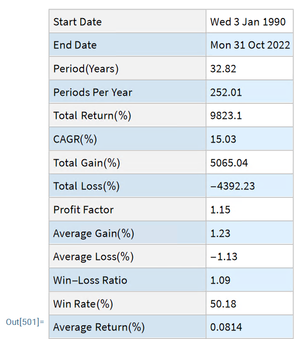
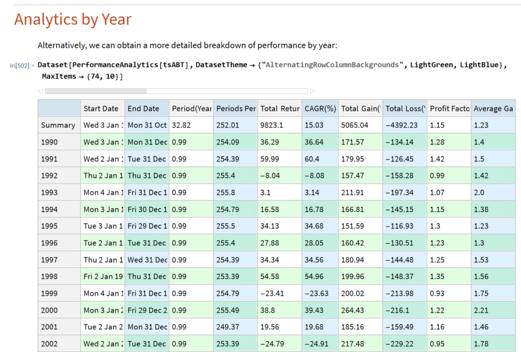
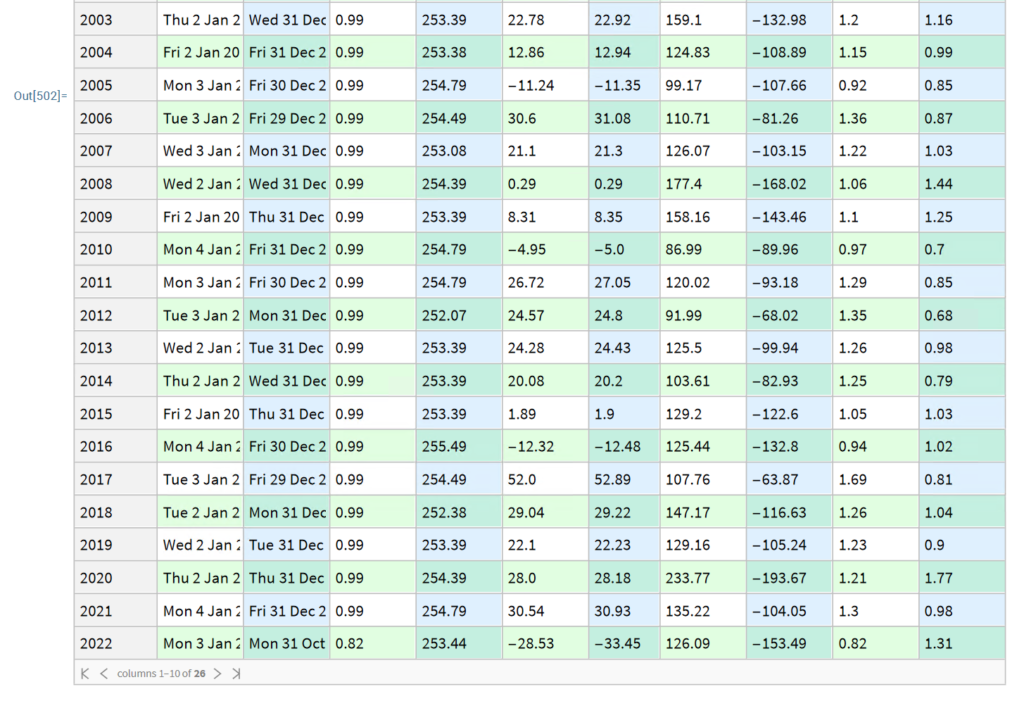
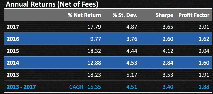
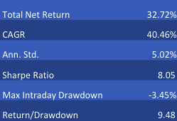
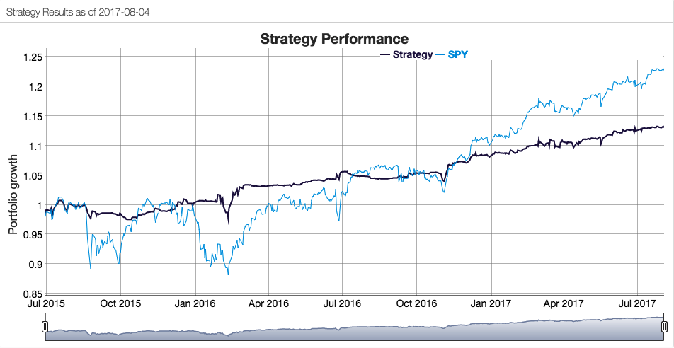
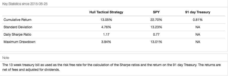
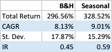
I am going to use an example our Quantitative Equity strategy, which forms part of the Systematic Strategies hedge fund. The tables and charts below give a broad impression of the performance characteristics of the strategy, which include a CAGR of 14.85% (net of fees) since live trading began in 2013.

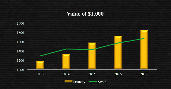
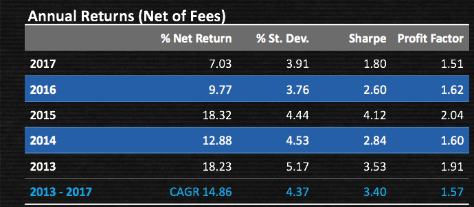
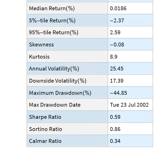
This is a strategy that is designed to produce returns on a par with the S&P 500 index, but with considerably lower risk: at just over 4%, the annual volatility of the strategy is only around 1/3 that of the index, while the maximum drawdown has been a little over 2% since inception. This level of portfolio risk is much lower than can typically be achieved in an equity long/short strategy (equity market neutral is another story, of course). Furthermore, the realized information ratio of 3.4 is in the upper 1%-tile of risk-adjusted performance amongst equity long/short strategies. So something rather more interesting must be going on that is very different from the typical approach to long/short equity.

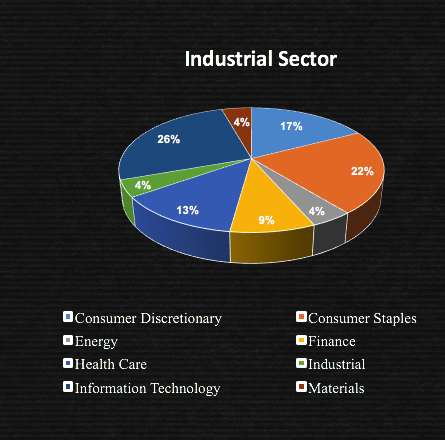
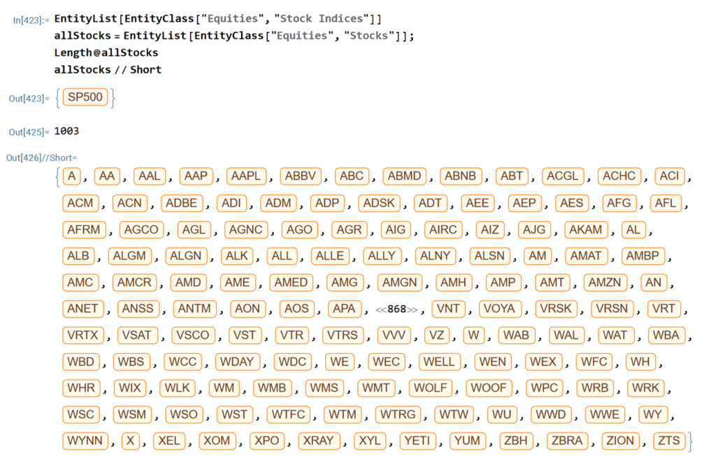
One plausible explanation is that the strategy is exploiting some minor market anomaly that works fine for small amounts of capital, but which cannot be scaled. But this is not the case here: the investment universe comprises more than a hundred of the most liquid stocks in US markets, across a broad spectrum of sectors. And while single-name investment is capped at 10% of average daily volume, this nonetheless provides investment capacity of several hundreds of millions of dollars.

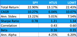
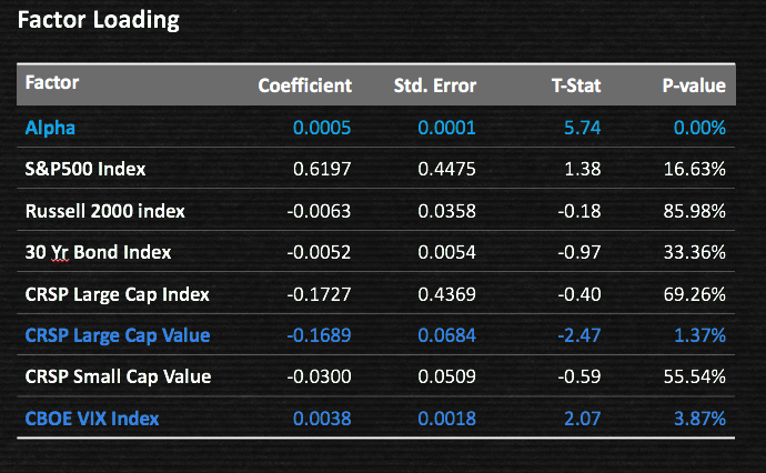
Nor does the reason for the exceptional performance lie in some new portfolio construction technique: rather, we rely on a straightforward 1/n allocation. Again, neither is factor exposure the driver of strategy alpha: as the factor loading table illustrates, strategy performance is largely uncorrelated with most market indices. It loads significantly on only large cap value, chiefly because the investment universe is defined as comprising the stocks with greatest liquidity (which tend to be large cap value), and on the CBOE VIX index. The positive correlation with market volatility is a common feature of many types of trading strategy that tend to do better in volatile markets, when short-term investment opportunities are plentiful.

While the detail of the strategy must necessarily remain proprietary, I can at least offer some insight that will, I hope, provide food for thought.

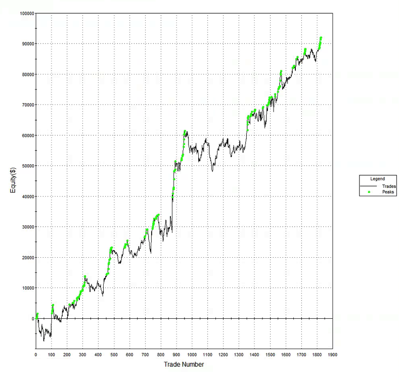
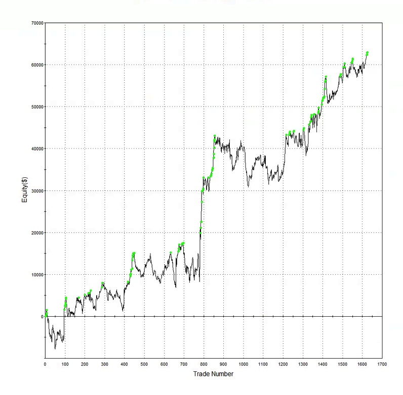
We can begin by comparing the returns for two of the stocks in the portfolio, Home Depot and Pfizer. The charts demonstrate one of important strategy characteristic: not every stock is traded at the same frequency. Some stocks might be traded once or twice a month; others possibly ten times a day, or more. In other words, the overall strategy is diversified significantly, not only across assets, but also across investment horizons. This has a considerable impact on volatility and downside risk in the portfolio.

Home Depot vs. Pfizer Inc.

Overall, the strategy trades an average of 40-60 times a day, or more. This is, admittedly, towards the low end of the frequency spectrum of HFT strategies – we might describe it as mid-frequency rather than high frequency trading. Nonetheless, compared to traditional long/short equity strategies this constitutes a high level of trading activity which, in aggregate, replicates some of the time-diversification benefits of HFT strategies, producing lower strategy volatility.

There is another way in which the strategy mimics, at least partially, the characteristics of a HFT strategy. The profitability of many (although by no means all) HFT strategies lies in their ability to capture (or, at least, not pay) the bid-offer spread. That is why latency is so crucial to most HFT strategies – if your aim is to to earn rebates, and/or capture the spread, you must enter and exit, passively, often using microstructure models to determine when to lean on the bid or offer price. That in turn depends on achieving a high priority for your orders in the limit order book, which is a function of latency – you need to be near the top of the queue at all times in order the achieve the required fill rate.

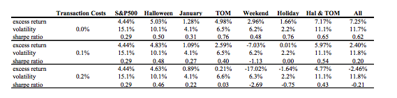
How does that apply here? While we are not looking to capture the spread, the strategy does seek to avoid taking liquidity and paying the spread. Where it can do so, it will offset the bid-offer spread by earning rebates. In many cases we are able to mitigate the spread cost altogether. So, while it cannot accomplish what a HFT market-making system can achieve, it can mimic enough of its characteristics – even at low frequency – to produce substantial gains in terms of cost-reduction and return enhancement. This is important since the transaction volume and portfolio turnover in this approach are significantly greater than for a typical equity long/short strategy.

Portfolio of Strategies vs. Portfolio of Equities

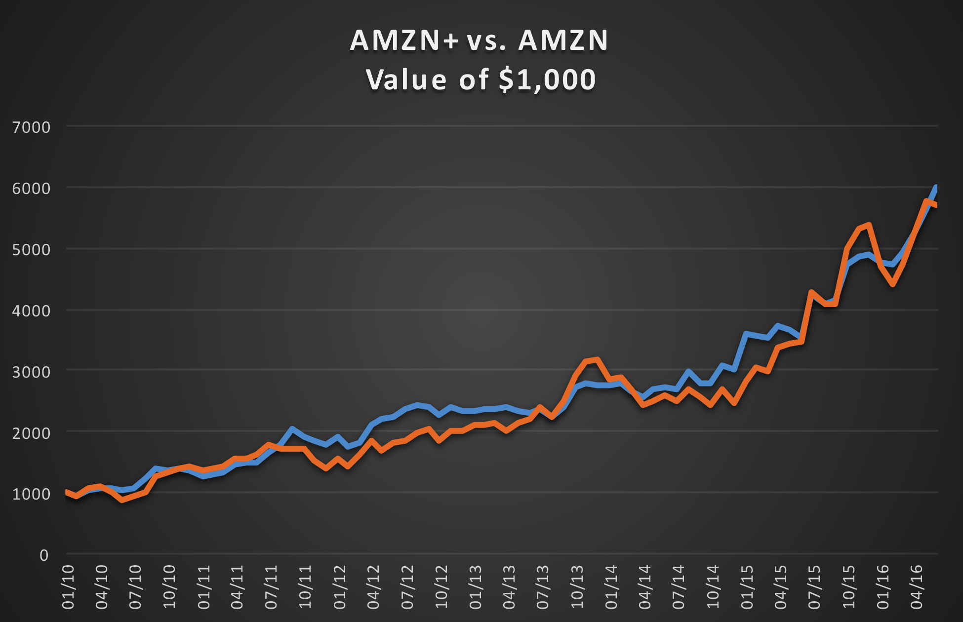
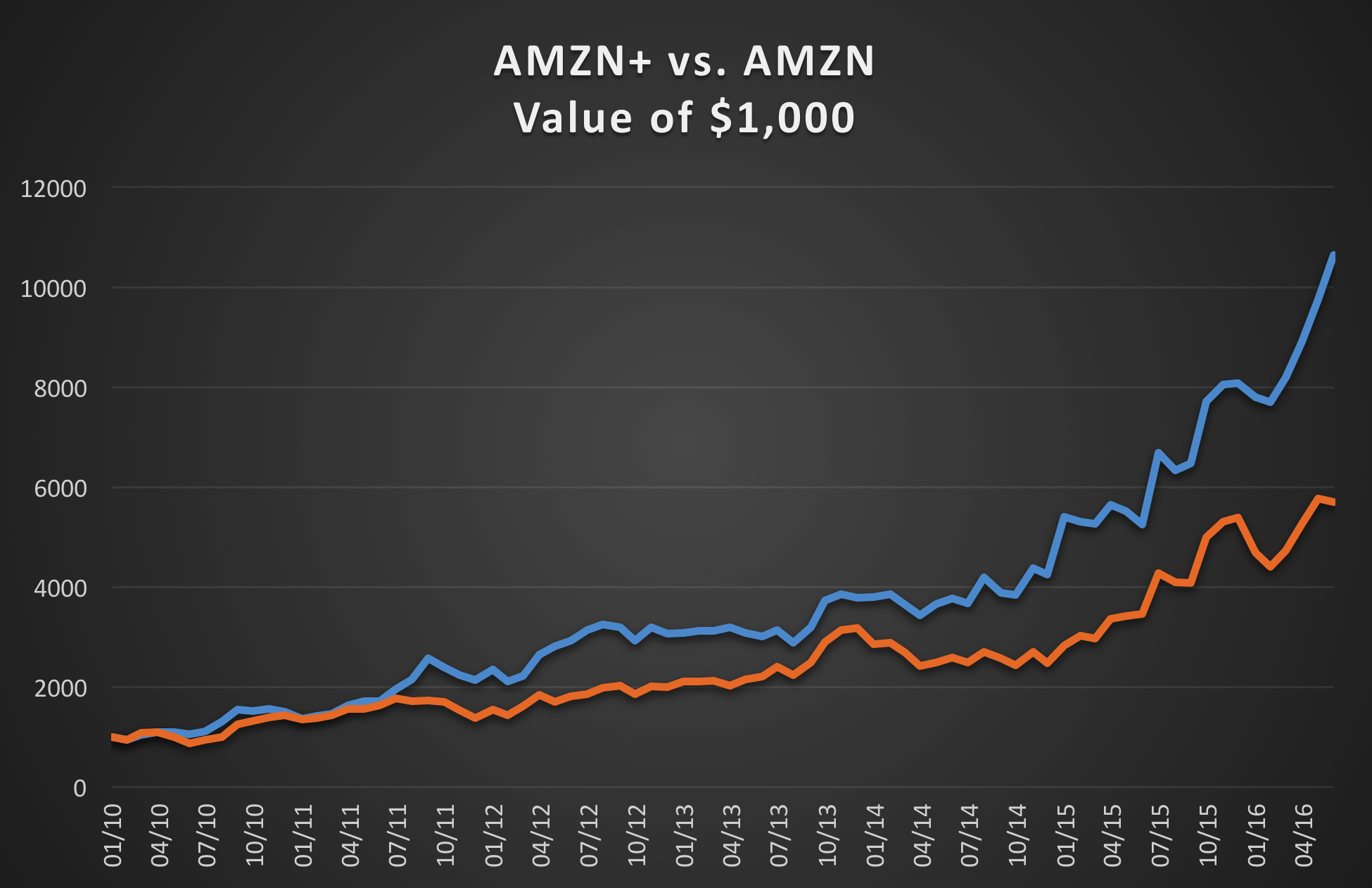
But this feature, while important, is not really the heart of the matter. Rather, the central point is this: that the overall strategy is an assembly of individual, independent strategies for each component stock. And it turns out that the diversification benefit of a portfolio of strategies is generally far greater than for an equal number of stocks, because the equity processes themselves will typically be correlated to a far greater degree than will corresponding trading strategies. To take the example of the pair of stocks discussed earlier, we find that the correlation between HD and PFE over the period from 2013 to 2017 is around 0.39, based on daily returns. By comparison, the correlation between the strategies for the two stocks over the same period is only 0.01.

This is generally the case, so that a portfolio of, say, 30 equity strategies, might reasonably be expected to enjoy a level of risk that is perhaps as much as one half that of a portfolio of the underlying stocks, no matter how constructed. This may be due to diversification in the time dimension, coupled with differences in the alpha generation mechanisms of the underlying strategies – mean reversion vs. momentum, for example

Strategy Robustness Testing

There are, of course, many different aspects to our approach to strategy risk management. Some of these are generally applicable to strategies of all varieties, but there are others that are specific to this particular type of strategy.

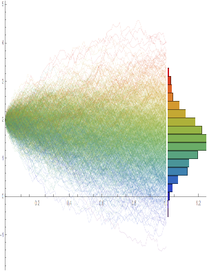
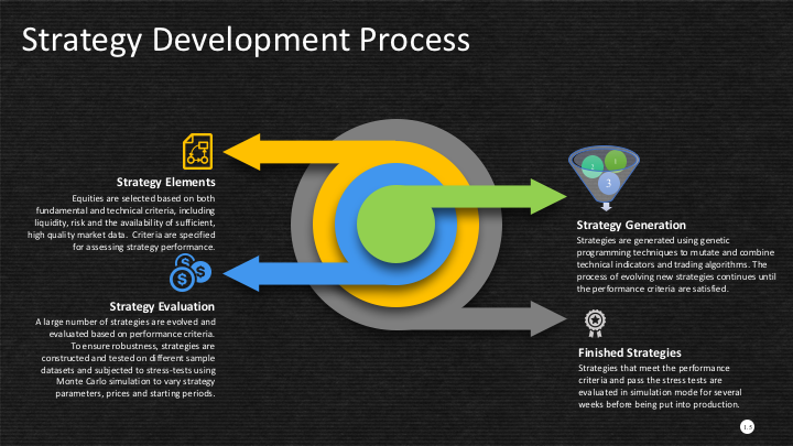
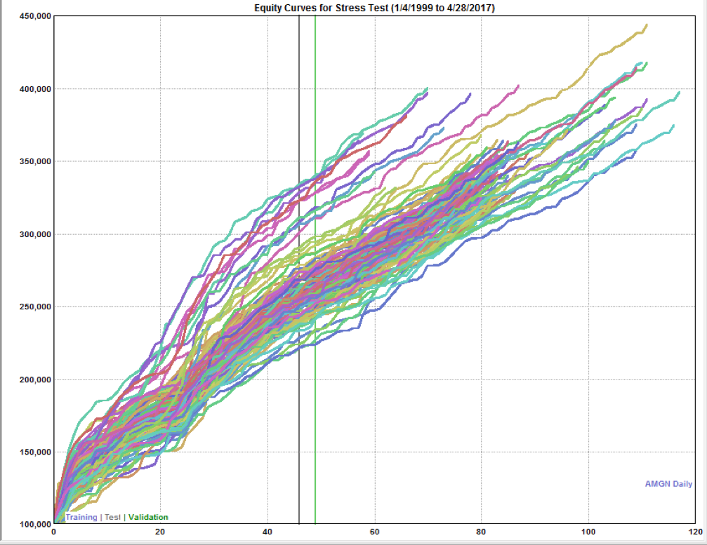
A good example of the latter is how we address the issue of strategy robustness. One of the principal concerns that investors have about quantitive strategies is that they may under-perform during adverse market conditions, or even simply stop working altogether. Our approach is to stress test each of the sub-strategy models using Monte Carlo simulation and examine their performance under a wide range of different scenarios, many of which have never been seen in the historical data used to construct the models.

For instance, we typically allow prices to fluctuate randomly by +/- 30% from historical values. But we also randomize the start date of each strategy by up to a year, which reduces the likelihood of a strategy being selected simply on the strength of a lucky start. Finally, we are interested in ensuring that the performance of each sub-strategy is not overly sensitive to the specific parameter values chosen for each model. Again, we test this using Monte Carlo, assessing the performance of each sub-strategy if the parameter values of the model are varied randomly by up to 30%.

The output of all these simulation tests is compiled into a histogram of performance results, from which we select the worst 5%-tile. Only if the worst outcomes – the 1-in-20 results in the left tail of the performance distribution – meet our performance criteria will the sub-strategy advance to the next stage of evaluation, simulated trading. This gives us – and investors – a level of confidence in the ability of the strategy to continue to perform well regardless of how market conditions evolve over time.

An obvious question to ask at this point is: if this is such a great idea, why don’t more firms use this approach? The answer is simple: it involves too much research. In a typical portfolio strategy there is a single investment idea that is applied cross-sectionally to a universe of stocks (factor models, momentum models, etc). In the strategy portfolio approach, separate strategies must be developed for each stock individually, which takes far more time and effort. Consequently such strategies must necessarily scale more slowly.

Another downside to the strategy portfolio approach is that it is less able to control the portfolio characteristics. For instance, the overall portfolio may, on average, have a beta close to zero; but there are likely to be times when a majority of the individual stock strategies align, producing a significantly higher, or lower, beta. The key here is to ask the question: what matters more – the semblance of risk control, or the actual risk characteristics of the strategy? In reality, the risk controls of traditional long/short equity strategies often turn out to be more theoretical than real. Time and again investors have seen strategies that turn out to be downside-correlated with the market, regardless of the purported “market-neutral” characteristics of the portfolio. I would argue that what matters far more is how the strategy actually performs under conditions of market stress, regardless of how “market neutral” or “sector neutral” it may purport to be. And while I agree that this is hardly a widely-held view, my argument would be that one cannot expect to achieve above-average performance simply by employing standard approaches at every turn.

Parallels with Fund of Funds Investment

So, is this really a “new approach” to equity long/short? Actually, no. It is certainly unusual. But it follows quite closely the model of a proprietary trading firm, or a Fund of Funds. There, as here, the task is to create a combined portfolio of strategies (or managers), rather than by investing directly in the underlying assets. A Fund of Funds will seek to create a portfolio of strategies that have low correlations to one another, and may operate a meta-strategy for allocating capital to the component strategies, or managers. But the overall investment portfolio cannot be as easily constrained as an individual equity portfolio can be – greater leeway must be allowed for the beta, or the dollar imbalance in the longs and shorts, to vary from time to time, even if over the long term the fluctuations average out. With human managers one always has to be concerned about the risk of “style drift” – i.e. when managers move away from their stated investment mandate, methodologies or objectives, resulting in a different investment outcomes. This can result in changes in the correlation between a strategy and its peers, or with the overall market. Quantitative strategies are necessarily more consistent in their investment approach – machines generally don’t alter their own source code – making a drift in style less likely. So an argument can be made that the risk inherent in this form of equity long/short strategy is on a par with – certainly not greater than – that of a typical fund of funds.

Conclusions

An investment approach that seeks to create a portfolio of strategies, rather than of underlying assets, offers a significant advantage in terms of risk reduction and diversification, due to the relatively low levels of correlation between the component strategies. The trading costs associated with higher frequency trading can be mitigated using passive entry/exit rules designed to avoid taking liquidity and generating exchange rebates. The downside is that it is much harder to manage the risk attributes of the portfolio, such as the portfolio beta, sector risk, or even the overall net long/short exposure. But these are indicators of strategy risk, rather than actual risk itself and they often fail to predict the actual risk characteristics of the strategy, especially during conditions of market stress. Investors may be better served by an approach to long/short equity that seeks to maximize diversification on the temporal axis as well as in terms of the factors driving strategy alpha.

Disclaimer: past performance does not guarantee future results. You should not rely on any past performance as a guarantee of future investment performance. Investment returns will fluctuate. Investment monies are at risk and you may suffer losses on any investment.

December 10, 2019

Modeling Asset Processes

Introduction

Over the last twenty five years significant advances have been made in the theory of asset processes and there now exist a variety of mathematical models, many of them computationally tractable, that provide a reasonable representation of their defining characteristics.

While the Geometric Brownian Motion model remains a staple of stochastic calculus theory, it is no longer the only game in town. Other models, many more sophisticated, have been developed to address the shortcomings in the original. There now exist models that provide a good explanation of some of the key characteristics of asset processes that lie beyond the scope of models couched in a simple Gaussian framework. Features such as mean reversion, long memory, stochastic volatility, jumps and heavy tails are now readily handled by these more advanced tools.

In this post I review a critical selection of asset process models that belong in every financial engineer’s toolbox, point out their key features and limitations and give examples of some of their applications.

Modeling Asset Processes

November 19, 2019

Strategy Portfolio Construction

July 30, 2019July 30, 2019

The Amazon Killer

Amazon (NASDAQ:AMZN) has been on a tear over the last decade, especially since the financial crisis of 2008. If you had been smart (or lucky) enough to buy the stock at the beginning of 2010, each $1,000 you invested would now be worth over $5,700, giving a CAGR of over 31%.

Source: Yahoo! Finance

It’s hard to argue with success, but could you have done better? The answer, surprisingly, is yes – and by a wide margin.

Introducing AMZN+

I am going to reveal this mystery stock in due course and, I promise you, the investment recommendation is fully actionable. For now, let’s just refer to it as AMZN+.

A comparison between investments made in AMZN and AMZN+ over the period from January 2010 to June 2016 is shown the chart following.

Visually, there doesn’t appear to be much of a difference in overall performance. However, it is apparent that AMZN+ is a great deal less volatile than its counterpart.

The table below give a more telling account of the relative outperformance by AMZN+.

The two investments are very highly correlated, with AMZN+ producing an extra 1% per annum in CAGR over the 6 ½ year period.

The telling distinction, however, lies on the risk side of the equation. Here AMZN+ outperforms AMZN by a wide margin, with an annual standard deviation of only 21% compared to 29%. What this means is that AMZN+ produces almost a 50% higher return than AMZN per unit of risk (information ratio 1.51 vs. 1.07).

The more conservative risk profile of AMZN+ is also reflected in lower maximum drawdown (-13.43% vs -23.74%), semi-deviation and higher Sortino Ratio (see this article for an explanation of these terms).

Bottom line: you can produce around the same rate of return with substantially less risk by investing in AMZN+, rather than AMZN.

Comparing Equally Risky Investments

There is another way to make the comparison, which some investors might find more appealing. Risk is, after all, an altogether more esoteric subject than return, which every investor understands.

So let’s say the investor adopts the same risk budget as for his original investment in AMZN, i.e. an annual volatility of just over 29%. We can produce the same overall level of risk in AMZN+, equalizing the riskiness of the two investments, simply by leveraging the investment in AMZN+ by a factor of 1.36, using margin money. i.e. we borrow $360 and invest a total of $1,360 in AMZN+, for each $1,000 we would have invested in AMZN. Look at the difference in performance:

The investor’s total return in AMZN+ would have been 963%, almost double the return in AMZN over the same period and with a CAGR of over 44.5%, more than 13% per annum higher than AMZN.

Note that, despite having an almost identical annual standard deviation, AMZN+ still enjoys a lower maximum drawdown and downside risk than AMZN.

The Big Reveal

Ok, so what is this mystery stock, AMZN+? Actually it isn’t a stock: it’s a simple portfolio, rebalanced monthly, with 66% of the investment being made in AMZN and 34% in the Direxion Daily 20+ Yr Trsy Bull 3X ETF (NYSEArca: TMF).

Well, that’s a little bit of a cheat, although not much of one: it isn’t too much of a challenge to put $667 of every $1,000 in AMZN and the remaining $333 in TMF, rebalancing the portfolio at the end of every month.

The next question an investor might want to ask is: what other stocks could I apply this approach to? The answer is: a great many of them. And where you end up, ultimately, is with the discovery that you can eliminate a great deal of unnecessary risk with a portfolio of around 20-30 well-chosen assets.

The Fundamental Lesson from Portfolio Theory

We saw that AMZN incurred a risk of 29% in annual standard deviation, compared to only 21% for the AMZN+ portfolio. What does the investor gain by taking that extra 8% in annual risk? Nothing at all – in fact he would have achieved a slightly worse return.

The key take-away from this simple example is the fundamental law of modern portfolio theory:

The market will not compensate an investor for taking diversifiable risk

As they say, diversification is the only free lunch on Wall Street. So make the most of it.

June 25, 2019

Seasonal Effects in Equity Markets

There are a plethora of seasonal anomalies documented in academic research. For equities these include the Halloween effect (“Sell in May”), January effect, turn-of-the-month effect, weekend effect and holiday effect. For example, Bouman and Jacobsen (2002) and Jacobsen and Visaltanachoti (2009) provide empirical evidence on the Halloween effect, Haug and Hirschey (2006) on the January effect, Lakonishok and Smidt (1988) on the turn-of-the-month (TOM) effect, Cross (1973) on the weekend effect, and Ariel (1990) on the holiday effect.

An excellent paper entitled An Anatomy of Calendar Effects in the Journal of Asset Management (13(4), 2012, pp. 271-286) by Laurens Swinkels of Erasmus University Rotterdam and Pim van Vliet of Robeco Asset Management gives a very good account of the various phenomena and their relative importance. Using daily returns data on the US value-weighted equity market over the period from July 1963 to December 2008, the researchers find that Halloween and turn-of-the-month (TOM) are the strongest effects, fully diminishing the other three effects to zero. The equity premium over the sample 1963-2008 is 7.2% if there is a Halloween or TOM effect, and -2.8% in all other cases. These findings are robust with respect to transactions costs, across different samples, market segments, and international stock markets. Their empirical research narrows down the number of calendar effects from five to two, leading to a more powerful and puzzling summary of seasonal effects.

The two principal effects are illustrated here with reference to daily returns in the S&P 500 Index, using data from 1980-2016.

Halloween Effect

The Halloween effect refers to the tendency of markets to perform better in the six month period from November to April, compared to the half year from May to October. In fact, for the S&P 500 index itself, performance during the months of May and October has historically been above the monthly average, as you can see in the chart below. According to this analysis, the period to avoid spans the four months from June to September, with September being the “cruelest month”, by far. Note that, between them, the months of November, December and April account for over 50% of the average annual return in the index since 1980.

Turn-of-the-Month Effect

The TOM effect refers to the finding that above average returns tend to occur on the last trading day of the month and (up to) the first four trading days of the new calendar month. For the S&P 500 index the TOM effect spans a shorter period comprising the last trading day of the month and the first two trading days of the new month. It is worth noting also the anomalous positive returns arising on 16th – 18th of the month and negative returns around the 19th and 20th of the month. My speculative guess is that these mid-month effects arise from futures/option expiration.

Seasonal Tactical Allocation

Let’s assume we allocate to equities (in the form of the S&P 500 Index) only during the period from October to May, or on the last or first two trading days of each month. How do the returns from that seasonal portfolio compare to the benchmark buy and hold portfolio? If we ignore transaction costs (and income from riskless Treasury investments when we are out of the market), the seasonal portfolio outperforms the buy and hold benchmark over the 36 year period since 1980 by around 88bp per annum (continuously compounded), and with an annual volatility that is 258bp lower. The outperformance of the seasonal portfolio becomes particularly noticeable after the 2000/2001 crash.

A much more rigorous analysis of the performance characteristics of the seasonal portfolio is given in the research paper, taking account of transaction costs, with summary results as follows:

Conclusion

There is a sizable body of credible academic research demonstrating the importance of calendar effects and this paper suggests that investors’ focus should be on the Halloween and TOM effects in particular. A tactical allocation program that increases the allocation to equities towards the end of the month and first few trading days of the new month, and during the November to April calendar months is likely to significantly outperform a buy-and-hold portfolio, according to these findings.

There remain unaccounted-for seasonal effects in the mid-section of the month that may arise from the expiration of futures and option contracts. These are worthy of further investigation.

May 21, 2019

High Frequency Trading: Equities vs. Futures

A talented young system developer I know recently reached out to me with an interesting-looking equity curve for a high frequency strategy he had designed in E-mini futures:

Pretty obviously, he had been making creative use of the “money management” techniques so beloved by futures systems designers. I invited him to consider how it would feel to be trading a 1,000-lot E-mini position when the market took a 20 point dive. A $100,000 intra-day drawdown might make the strategy look a little less appealing. On the other hand, if you had already made millions of dollars in the strategy, you might no longer care so much.

A more important criticism of money management techniques is that they are typically highly path-dependent: if you had started your strategy slightly closer to one of the drawdown periods that are almost unnoticeable on the chart, it could have catastrophic consequences for your trading account. The only way to properly evaluate this, I advised, was to backtest the strategy over many hundreds of thousands of test-runs using Monte Carlo simulation. That would reveal all too clearly that the risk of ruin was far larger than might appear from a single backtest.

Next, I asked him whether the strategy was entering and exiting passively, by posting bids and offers, or aggressively, by crossing the spread to sell at the bid and buy at the offer. I had a pretty good idea what his answer would be, given the volume of trades in the strategy and, sure enough he confirmed the strategy was using passive entries and exits. Leaving to one side the challenge of executing a trade for 1,000 contracts in this way, I instead ask him to show me the equity curve for a single contract in the underlying strategy, without the money-management enhancement. It was still very impressive.

The Critical Fill Assumptions For Passive Strategies

But there is an underlying assumption built into these results, one that I have written about in previous posts: the fill rate. Typically in a retail trading platform like Tradestation the assumption is made that your orders will be filled if a trade occurs at the limit price at which the system is attempting to execute. This default assumption of a 100% fill rate is highly unrealistic. The system’s orders have to compete for priority in the limit order book with the orders of many thousands of other traders, including HFT firms who are likely to beat you to the punch every time. As a consequence, the actual fill rate is likely to be much lower: 10% to 20%, if you are lucky. And many of those fills will be “toxic”: buy orders will be the last to be filled just before the market moves lower and sell orders will be the last to get filled just as the market moves higher. As a result, the actual performance of the strategy will be a very long way from the pretty picture shown in the chart of the hypothetical equity curve.

One way to get a handle on the problem is to make a much more conservative assumption, that your limit orders will only get filled when the market moves through them. This can easily be achieved in a product like Tradestation by selecting the appropriate backtest option:

The strategy performance results often look very different when this much more conservative fill assumption is applied. The outcome for this system was not at all unusual:

Of course, the more conservative assumption applied here is also unrealistic: many of the trading system’s sell orders would be filled at the limit price, even if the market failed to move higher (or lower in the case of a buy order). Furthermore, even if they were not filled during the bar-interval in which they were issued, many limit orders posted by the system would be filled in subsequent bars. But the reality is likely to be much closer to the outcome assuming a conservative fill-assumption than an optimistic one. Put another way: if the strategy demonstrates good performance under both pessimistic and optimistic fill assumptions there is a reasonable chance that it will perform well in practice, other considerations aside.

An Example of a HFT Equity Strategy

Let’s contrast the futures strategy with an example of a similar HFT strategy in equities. Under the optimistic fill assumption the equity curve looks as follows:

Under the more conservative fill assumption, the equity curve is obviously worse, but the strategy continues to produce excellent returns. In other words, even if the market moves against the system on every single order, trading higher after a sell order is filled, or lower after a buy order is filled, the strategy continues to make money.

Market Microstructure

There is a fundamental reason for the discrepancy in the behavior of the two strategies under different fill scenarios, which relates to the very different microstructure of futures vs. equity markets. In the case of the E-mini strategy the average trade might be, say, $50, which is equivalent to only 4 ticks (each tick is worth $12.50). So the average trade: tick size ratio is around 4:1, at best. In an equity strategy with similar average trade the tick size might be as little as 1 cent. For a futures strategy, crossing the spread to enter or exit a trade more than a handful of times (or missing several limit order entries or exits) will quickly eviscerate the profitability of the system. A HFT system in equities, by contrast, will typically prove more robust, because of the smaller tick size.

Of course, there are many other challenges to high frequency equity trading that futures do not suffer from, such as the multiplicity of trading destinations. This means that, for instance, in a consolidated market data feed your system is likely to see trading opportunities that simply won’t arise in practice due to latency effects in the feed. So the profitability of HFT equity strategies is often overstated, when measured using a consolidated feed. Futures, which are traded on a single exchange, don’t suffer from such difficulties. And there are a host of other differences in the microstructure of futures vs equity markets that the analyst must take account of. But, all that understood, in general I would counsel that equities make an easier starting point for HFT system development, compared to futures.

February 18, 2019February 18, 2019

Pairs Trading in Practice

Part 1 – Methodologies

It is perhaps a little premature for a deep dive into the Gemini Pairs Trading strategy which trades on our Systematic Algotrading platform. At this stage all one can say for sure is that the strategy has made a pretty decent start – up around 17% from October 2018. The strategy does trade multiple times intraday, so the record in terms of completed trades – numbering over 580 – is appreciable (the web site gives a complete list of live trades). And despite the turmoil through the end of last year the Sharpe Ratio has ranged consistently around 2.5.

One of the theoretical advantages of pairs trading is, of course, that the coupling of long and short positions in a relative value trade is supposed to provide a hedge against market downdrafts, such as we saw in Q4 2018. In that sense pairs trading is the quintessential hedge fund strategy, embodying the central concept on which the entire edifice of hedge fund strategies is premised.

In practice, however, things often don’t work out as they should. In this thread I want to spend a little time reviewing why that is and to offer some thoughts based on my own experience of working with statistical arbitrage strategies over many years.

Methodology

There is no “secret recipe” for pairs trading: the standard methodologies are as well known as the strategy concept. But there are some important practical considerations that I would like to delve into in this post. Before doing that, let me quickly review the tried and tested approaches used by statistical arbitrageurs.

The Ratio Model is one of the standard pair trading models described in literature. It is based in ratio of instrument prices, moving average and standard deviation. In other words, it is based on Bollinger Bands indicator.

we trade pair of stocks A, B, having price series A(t), B(t)
we need to calculate ratio time series R(t) = A(t) / B(t)
we apply a moving average of type T with period P_m on R(t) to get time series M(t)
Next we apply the standard deviation with period P_s on R(t) to get time series S(t)
now we can create Z-score series Z(t) as Z(t) = (R(t) – M(t)) / S(t), this time series can give us z-score to signal trading decision directly (in reality we have two Z-scores: Z-score_ask and Z-score_bid as they are calculated using different prices, but for the sake of simplicity let’s now pretend we don’t pay bid-ask spread and we have just one Z-score)

Another common way to visualize this approach is to think in terms of bands around the moving average M(t):

upper entry band U_n(t) = M(t) + S(t) * E_n
lower entry band L_n(t) = M(t) – S(t) * E_n
upper exit band U_x(t) = M(t) + S(t) * E_x
lower exit band L_x(t) = M(t) – S(t) * E_x

These bands are actually the same bands as in Bollinger Bands indicator and we can use crossing of R(t) and bands as trade signals.

We open short pair position, if the Z-score Z(t) >= E_n (equivalent to R(t) >= U_n(t))
We open long pair position if the Z-score Z(t) <= -E_n (equivalent to R(t) <= L_n(t))

In the Regression, Residual or Cointegration approach we construct a linear regression between A(t), B(t) using OLS, where A(t) = β * B(t) + α + R(t)

Because we use a moving window of period P (we calculate new regression each day), we actually get new series β(t), α(t), R(t), where β(t), α(t) are series of regression coefficients and R(t) are residuals (prediction errors)

We look at the residuals series R(t) = A(t) – (β(t) * B(t) + α(t))
We next calculate the standard deviation of the residuals R(t), which we designate S(t)
Now we can create Z-score series Z(t) as Z(t) = R(t) / S(t) – the time series that is used to generate trade signals, just as in the Ratio model.

The Kalman Filter model provides superior estimates of the current hedge ratio compared to the Regression method. For a detailed explanation of the techniques, see the following posts (the post on ETF trading contains complete Matlab code).

Finally, the rather complex Copula methodology models the joint and margin distributions of the returns process in each stock as described in the following post

January 11, 2019January 11, 2019

A Universal Stock Screening Application

Happy New Year to my readers.

I recently pitched a consulting project that entailed building a stock screener that would apply both fundamental and technical criteria to identity a universe of candidate stocks across world-wide equity markets.

Here is how I approached the task:

StockScreener_1_4