Part 1 – Methodologies
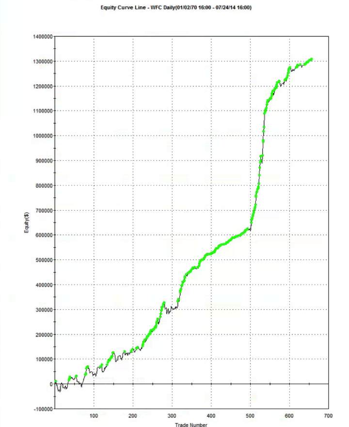
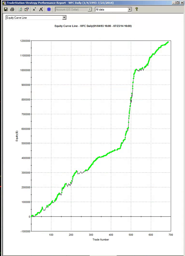
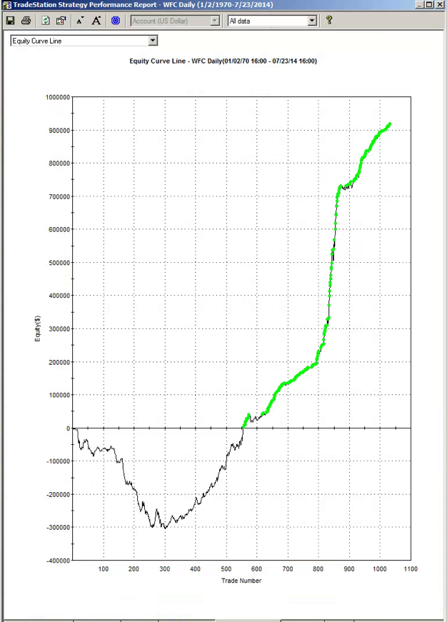
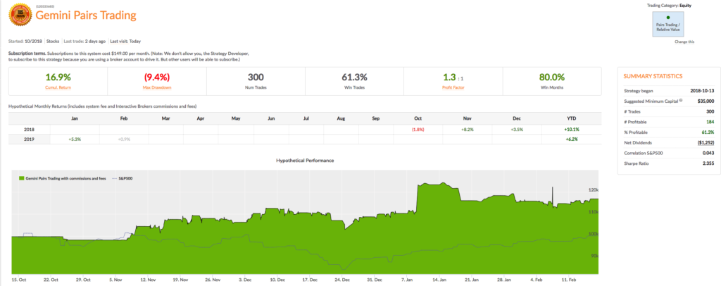
It is perhaps a little premature for a deep dive into the Gemini Pairs Trading strategy which trades on our Systematic Algotrading platform. At this stage all one can say for sure is that the strategy has made a pretty decent start – up around 17% from October 2018. The strategy does trade multiple times intraday, so the record in terms of completed trades – numbering over 580 – is appreciable (the web site gives a complete list of live trades). And despite the turmoil through the end of last year the Sharpe Ratio has ranged consistently around 2.5.
Methodology
There is no “secret recipe” for pairs trading: the standard methodologies are as well known as the strategy concept. But there are some important practical considerations that I would like to delve into in this post. Before doing that, let me quickly review the tried and tested approaches used by statistical arbitrageurs.
The Ratio Model is one of the standard pair trading models described in literature. It is based in ratio of instrument prices, moving average and standard deviation. In other words, it is based on Bollinger Bands indicator.
- we trade pair of stocks A, B, having price series A(t), B(t)
- we need to calculate ratio time series R(t) = A(t) / B(t)
- we apply a moving average of type T with period Pm on R(t) to get time series M(t)
- Next we apply the standard deviation with period Ps on R(t) to get time series S(t)
- now we can create Z-score series Z(t) as Z(t) = (R(t) – M(t)) / S(t), this time series can give us z-score to signal trading decision directly (in reality we have two Z-scores: Z-scoreask and Z-scorebid as they are calculated using different prices, but for the sake of simplicity let’s now pretend we don’t pay bid-ask spread and we have just one Z-score)
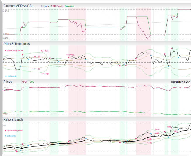
Another common way to visualize this approach is to think in terms of bands around the moving average M(t):
- upper entry band Un(t) = M(t) + S(t) * En
- lower entry band Ln(t) = M(t) – S(t) * En
- upper exit band Ux(t) = M(t) + S(t) * Ex
- lower exit band Lx(t) = M(t) – S(t) * Ex
These bands are actually the same bands as in Bollinger Bands indicator and we can use crossing of R(t) and bands as trade signals.
- We open short pair position, if the Z-score Z(t) >= En (equivalent to R(t) >= Un(t))
- We open long pair position if the Z-score Z(t) <= -En (equivalent to R(t) <= Ln(t))
In the Regression, Residual or Cointegration approach we construct a linear regression between A(t), B(t) using OLS, where A(t) = β * B(t) + α + R(t)
Because we use a moving window of period P (we calculate new regression each day), we actually get new series β(t), α(t), R(t), where β(t), α(t) are series of regression coefficients and R(t) are residuals (prediction errors)
- We look at the residuals series R(t) = A(t) – (β(t) * B(t) + α(t))
- We next calculate the standard deviation of the residuals R(t), which we designate S(t)
- Now we can create Z-score series Z(t) as Z(t) = R(t) / S(t) – the time series that is used to generate trade signals, just as in the Ratio model.
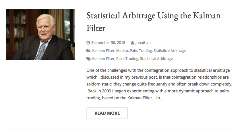
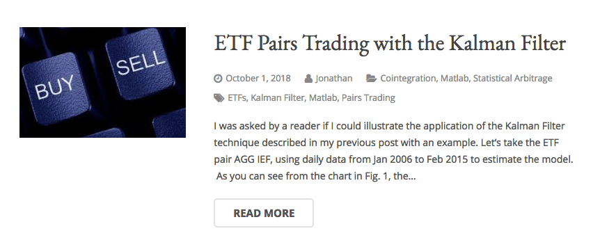
The Kalman Filter model provides superior estimates of the current hedge ratio compared to the Regression method. For a detailed explanation of the techniques, see the following posts (the post on ETF trading contains complete Matlab code).
Finally, the rather complex Copula methodology models the joint and margin distributions of the returns process in each stock as described in the following post