A follow-up extract from my forthcoming book, Equity Analytics
Applying-Factor-Models-in-Pairs-TradingPairs Trading in the Equities Entity Store
An extract from the chapter on pairs trading from my forthcoming book Equity Analytics
Pairs-Trading-1A Practical Application of Regime Switching Models to Pairs Trading
In the previous post I outlined some of the available techniques used for modeling market states. The following is an illustration of how these techniques can be applied in practice. You can download this post in pdf format here.
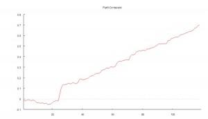
The chart below shows the daily compounded returns for a single pair in an ETF statistical arbitrage strategy, back-tested over a 1-year period from April 2010 to March 2011.
The idea is to examine the characteristics of the returns process and assess its predictability.
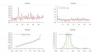
The initial impression given by the analytics plots of daily returns, shown in Fig 2 below, is that the process may be somewhat predictable, given what appears to be a significant 1-order lag in the autocorrelation spectrum. We also see evidence of the
customary non-Gaussian “fat-tailed” distribution in the error process.
An initial attempt to fit a standard Auto-Regressive Moving Average ARMA(1,0,1) model yields disappointing results, with an unadjusted model R-squared of only 7% (see model output in Appendix 1)
However, by fitting a 2-state Markov model we are able to explain as much as 65% in the variation in the returns process (see Appendix II).
The model estimates Markov Transition Probabilities as follows.
P(.|1) P(.|2)
P(1|.) 0.93920 0.69781
P(2|.) 0.060802 0.30219
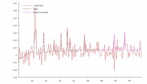
In other words, the process spends most of the time in State 1, switching to State 2 around once a month, as illustrated in Fig 3 below.
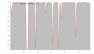
In the first state, the pairs model produces an expected daily return of around 65bp, with a standard deviation of similar magnitude. In this state, the process also exhibits very significant auto-regressive and moving average features.
Regime 1:
Intercept 0.00648 0.0009 7.2 0
AR1 0.92569 0.01897 48.797 0
MA1 -0.96264 0.02111 -45.601 0
Error Variance^(1/2) 0.00666 0.0007
In the second state, the pairs model produces lower average returns, and with much greater variability, while the autoregressive and moving average terms are poorly determined.
Regime 2:
Intercept 0.03554 0.04778 0.744 0.459
AR1 0.79349 0.06418 12.364 0
MA1 -0.76904 0.51601 -1.49 0.139
Error Variance^(1/2) 0.01819 0.0031
CONCLUSION
The analysis in Appendix II suggests that the residual process is stable and Gaussian. In other words, the two-state Markov model is able to account for the non-Normality of the returns process and extract the salient autoregressive and moving average features in a way that makes economic sense.
How is this information useful? Potentially in two ways:
(i) If the market state can be forecast successfully, we can use that information to increase our capital allocation during periods when the process is predicted to be in State 1, and reduce the allocation at times when it is in State 2.
(ii) By examining the timing of the Markov states and considering different features of the market during the contrasting periods, we might be able to identify additional explanatory factors that could be used to further enhance the trading model.
Learning the Kalman Filter
Michael Kleder’s “Learning the Kalman Filter” mini tutorial, along with the great feedback it has garnered (73 comments and 67 ratings, averaging 4.5 out of 5 stars), is one of the most popular downloads from Matlab Central and for good reason.
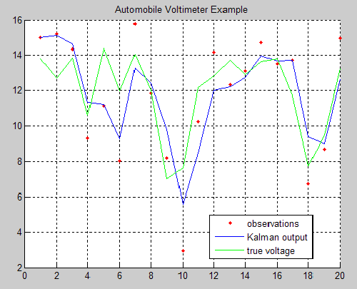
In his in-file example, Michael steps through a Kalman filter example in which a voltmeter is used to measure the output of a 12-volt automobile battery. The model simulates both randomness in the output of the battery, and error in the voltmeter readings. Then, even without defining an initial state for the true battery voltage, Michael demonstrates that with only 5 lines of code, the Kalman filter can be implemented to predict the true output based on (not-necessarily-accurate) uniformly spaced, measurements:
This is a simple but powerful example that shows the utility and potential of Kalman filters. It’s sure to help those who are trepid about delving into the world of Kalman filtering.
Successful Statistical Arbitrage
I tend not to get involved in Q&A with readers of my blog, or with investors. I am at a point in my life where I spend my time mostly doing what I want to do, rather than what other people would like me to do. And since I enjoy doing research and trading, I try to maximize the amount of time I spend on those activities.
As a business strategy, I wouldn’t necessarily recommend this approach. It’s just something I evolved while learning to play chess: since I had no-one to teach me, I had to learn everything for myself and this involved studying for many, many hours alone.
By contrast, several of the best money managers are also excellent communicators – take Roy Niederhoffer, or Ernie Chan, for example. Having regular, informed communication with your investors is, as smarter managers have realized, a means of building trust and investor loyalty – important factors that come into play during periods when your strategy is underperforming. Not only that, but since communication is two-way, an analyst/manager can learn much from his exchanges with his clients. Knowing how others perceive you – and your competitors – for example, is very useful information. So, too, is information about your competitors’ research ideas, investment strategies and fund performance, which can often be gleaned from discussions with investors. There are plenty of reasons to prefer a policy of regular, open communication.
As a case in point, I was surprised to learn from comments on another research blog that readers drew the conclusion from my previous posts that pursuing the cointegration or Kalman Filter approach to statistical arbitrage was a waste of time. Apparently, my remark to the effect that researchers often failed to pay attention to the net PnL per share in evaluating stat. arb. trading strategies was taken by some to mean that any apparent profitability would always be subsumed within the bid-offer spread. That was not my intention. What I intended to convey was that in some instances, this would be the case – some, but not all.
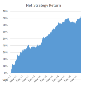
To illustrate the point, below are the out-of-sample results from a research study applying the Kalman Filter approach for four equity pairs using 5-minute data. For competitive reasons I am unable to identify the specific stocks in each pair, which result from an exhaustive analysis of over 30,000 pairs, but I can say that they are liquid large-cap equities traded in large volume on the US exchanges. The performance numbers are net of transaction costs and are based on the assumption of a 5-minute delay in execution: meaning, a trading signal received at time t is assumed to be executed at time t+5 minutes. This allows sufficient time to leg into each trade passively, in most cases avoiding the bid-offer spread. The net PnL per share is above 1.5c per share for each pair.
 While the performance of none of the pairs is spectacular, a combined portfolio has quite attractive characteristics, which include 81% winning months since Jan 2012, a CAGR of over 27% and Information Ratio of 2.29, measured on monthly returns (2.74 based on daily returns).
Finally, I am currently implementing trading of a number of stock portfolios based on static cointegration relationships that have out-of-sample information ratios of between 3 and 4, using daily data.
ETF Pairs Trading with the Kalman Filter
I was asked by a reader if I could illustrate the application of the Kalman Filter technique described in my previous post with an example. Let’s take the ETF pair AGG IEF, using daily data from Jan 2006 to Feb 2015 to estimate the model. As you can see from the chart in Fig. 1, the pair have been highly correlated over the last several years.
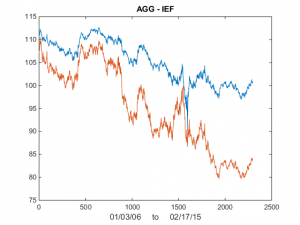 Fig 1. AGG and IEF Daily Prices 2006-2015
We now estimate the beta-relationship between the ETF pair with the Kalman Filter, using the Matlab code given below, and plot the estimated vs actual prices of the first ETF, AGG in Fig 2. There are one or two outliers that you might want to take a look at, but mostly the fit looks very good. 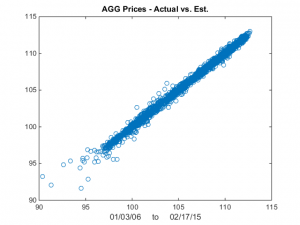
Fig 2 – Actual vs Fitted Prices of AGG
Now lets take a look at Kalman Filter estimates of beta. As you can see in Fig 3, it wanders around a lot! Very difficult to handle using some kind of static beta estimate. 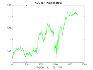
Fig 3 – Kalman Filter Beta Estimates
Finally, we compute the raw and standardized alphas, being the differences between the observed and fitted prices , i.e. Alpha(t) = AGG(t) – b(t)* IEF(t) and kfAlpha(t) = (Alpha(t) – mean(Alpha(t)) / std(Alpha(t) I have plotted the kfAlpha estimates over the last year in Fig 4. 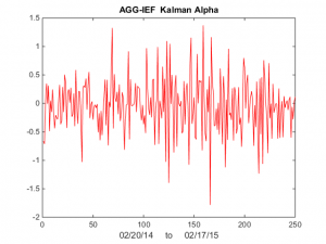
Fig 4 – Standardized Alpha Estimates
The last step is to decide how to trade this relationship. You might, for example, trade the portfolio in proportion to the standardized deviation (i.e. the size of kfAlpha(t)). Alternatively, you might set a threshold level, say +/- 1 Sd, and trade the portfolio when kfAlpha(t) exceeds this the threshold. In the Matlab code below I use the particle swarm method to maximize the likelihood. I have found this to be more reliable than other methods.
Statistical Arbitrage Using the Kalman Filter
One of the challenges with the cointegration approach to statistical arbitrage which I discussed in my previous post, is that cointegration relationships are seldom static: they change quite frequently and often break down completely. Back in 2009 I began experimenting with a more dynamic approach to pairs trading, based on the Kalman Filter.
In its simplest form, we model the relationship between a pair of securities in the following way:
beta(t) = beta(t-1) + w beta(t), the unobserved state variable, that follows a random walk
Y(t) = beta(t)X(t) + v The observed processes of stock prices Y(t) and X(t)
where:
w ~ N(0,Q) meaning w is gaussian noise with zero mean and variance Q
v ~ N(0,R) meaning v is gaussian noise with variance R
So this is just like the usual pairs relationship Y = beta * X + v, where the typical approach is to estimate beta using least squares regression, or some kind of rolling regression (to try to take account of the fact that beta may change over time). In this traditional framework, beta is static, or slowly changing.
In the Kalman framework, beta is itself a random process that evolves continuously over time, as a random walk. Because it is random and contaminated by noise we cannot observe beta directly, but must infer its (changing) value from the observable stock prices X and Y. (Note: in what follows I shall use X and Y to refer to stock prices. But you could also use log prices, or returns).
Unknown to me at that time, several other researchers were thinking along the same lines and later published their research. One such example is Statistical Arbitrage and High-Frequency Data with an Application to Eurostoxx 50 Equities, Rudy, Dunis, Giorgioni and Laws, 2010. Another closely related study is Performance Analysis of Pairs Trading Strategy Utilizing High Frequency Data with an Application to KOSPI 100 Equities, Kim, 2011. Both research studies follow a very similar path, rejecting beta estimation using rolling regression or exponential smoothing in favor of the Kalman approach and applying a Ornstein-Uhlenbeck model to estimate the half-life of mean reversion of the pairs portfolios. The studies report very high out-of-sample information ratios that in some cases exceed 3.
I have already made the point that such unusually high performance is typically the result of ignoring the fact that the net PnL per share may lie within the region of the average bid-offer spread, making implementation highly problematic. In this post I want to dwell on another critical issue that is particular to the Kalman approach: the signal:noise ratio, Q/R, which expresses the ratio of the variance of the beta process to that of the price process. (Curiously, both papers make the same mistake of labelling Q and R as standard deviations. In fact, they are variances).
Beta, being a random process, obviously contains some noise: but the hope is that it is less noisy than the price process. The idea is that the relationship between two stocks is more stable – less volatile – than the stock processes themselves. On its face, that assumption appears reasonable, from an empirical standpoint. The question is: how stable is the beta process, relative to the price process? If the variance in the beta process is low relative to the price process, we can determine beta quite accurately over time and so obtain accurate estimates of the true price Y(t), based on X(t). Then, if we observe a big enough departure in the quoted price Y(t) from the true price at time t, we have a potential trade.
In other words, we are interested in:
alpha(t) = Y(t) – Y*(t) = Y(t) – beta(t) X(t)
where Y(t) and X(t) are the observed stock prices and beta(t) is the estimated value of beta at time t.
As usual, we would standardize the alpha using an estimate of the alpha standard deviation, which is sqrt(R). (Alternatively, you can estimate the standard deviation of the alpha directly, using a lookback period based on the alpha half-life).
If the standardized alpha is large enough, the model suggests that the price Y(t) is quoted significantly in excess of the true value. Hence we would short stock Y and buy stock X. (In this context, where X and Y represent raw prices, you would hold an equal and opposite number of shares in Y and X. If X and Y represented returns, you would hold equal and opposite market value in each stock).
The success of such a strategy depends critically on the quality of our estimates of alpha, which in turn rest on the accuracy of our estimates of beta. This depends on the noisiness of the beta process, i.e. its variance, Q. If the beta process is very noisy, i.e. if Q is large, our estimates of alpha are going to be too noisy to be useful as the basis for a reversion strategy.
So, the key question I want to address in this post is: in order for the Kalman approach to be effective in modeling a pairs relationship, what would be an acceptable range for the beta process variance Q ? (It is often said that what matters in the Kalman framework is not the variance Q, per se, but rather the signal:noise ratio Q/R. It turns out that this is not strictly true, as we shall see).
To get a handle on the problem, I have taken the following approach:
(i) Simulate a stock process X(t) as a geometric brownian motion process with specified drift and volatility (I used 0%, 5% and 10% for the annual drift, and 10%, 30% and 60% for the corresponding annual volatility).
(ii) simulate a beta(t) process as a random walk with variance Q in the range from 1E-10 to 1E-1.
(iii) Generate the true price process Y(t) = beta(t)* X(t)
(iv) Simulate an observed price process Yobs(t), by adding random noise with variance R to Y(t), with R in the range 1E-6 to 1.0
(v) Calculate the true, known alpha(t) = Y(t) – Yobs(t)
(vi) Fit the Kalman Filter model to the simulated processes and estimate beta(t) and Yest(t). Hence produce estimates kfalpha(t) = Yobs(t) – Yest(t) and compare these with the known, true alpha(t).
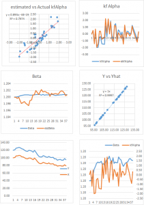
The charts in Fig. 1 below illustrate the procedure for a stock process X(t) with annual drift of 10%, annual volatility 40%, beta process variance Q of 8.65E-9 and price process variance R of 5.62E-2 (Q/R ratio of 1.54E-7).
Fig. 1 True and Estimated Beta and Alpha Using the Kalman Filter
As you can see, the Kalman Filter does a very good job of updating its beta estimate to track the underlying, true beta (which, in this experiment, is known). As the noise ratio Q/R is small, the Kalman Filter estimates of the process alpha, kfalpha(t), correspond closely to the true alpha(t), which again are known to us in this experimental setting. You can examine the relationship between the true alpha(t) and the Kalman Filter estimates kfalpha(t) is the chart in the upmost left quadrant of the figure. The correlation between the two is around 89%. With a level of accuracy this good for our alpha estimates, the pair of simulated stocks would make an ideal candidate for a pairs trading strategy.
Of course, the outcome is highly dependent on the values we assume for Q and R (and also to some degree on the assumptions made about the drift and volatility of the price process X(t)).
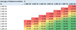
The next stage of the analysis is therefore to generate a large number of simulated price and beta observations and examine the impact of different levels of Q and R, the variances of the beta and price process. The results are summarized in the table in Fig 2 below.
Fig 2. Correlation between true alpha(t) and kfalpha(t) for values of Q and R
As anticipated, the correlation between the true alpha(t) and the estimates produced by the Kalman Filter is very high when the signal:noise ratio is small, i.e. of the order of 1E-6, or less. Average correlations begin to tail off very quickly when Q/R exceeds this level, falling to as low as 30% when the noise ratio exceeds 1E-3. With a Q/R ratio of 1E-2 or higher, the alpha estimates become too noisy to be useful.
I find it rather fortuitous, even implausible, that in their study Rudy, et al, feel able to assume a noise ratio of 3E-7 for all of the stock pairs in their study, which just happens to be in the sweet spot for alpha estimation. From my own research, a much larger value in the region of 1E-3 to 1E-5 is more typical. Furthermore, the noise ratio varies significantly from pair to pair, and over time. Indeed, I would go so far as to recommend applying a noise ratio filter to the strategy, meaning that trading signals are ignored when the noise ratio exceeds some specified level.
The take-away is this: the Kalman Filter approach can be applied very successfully in developing statistical arbitrage strategies, but only for processes where the noise ratio is not too large. One suggestion is to use a filter rule to supress trade signals generated at times when the noise ratio is too large, and/or to increase allocations to pairs in which the noise ratio is relatively low.
