Futures Archives - Page 3 of 4 - QUANTITATIVE RESEARCH AND TRADING

March 12, 2019

Overnight Trading in the E-Mini S&P 500 Futures

Jeff Swanson’s Trading System Success web site is often worth a visit for those looking for new trading ideas.

A recent post Seasonality S&P Market Session caught my eye, having investigated several ideas for overnight trading in the E-minis. Seasonal effects are of course widely recognized and traded in commodities markets, but they can also apply to financial products such as the E-mini. Jeff’s point about session times is well-made: it is often worthwhile to look at the behavior of an asset, not only in different time frames, but also during different periods of the trading day, day of the week, or month of the year.

Jeff breaks the E-mini trading session into several basic sub-sessions:

“Pre-Market” Between 530 and 830
“Open” Between 830 and 900
“Morning” Between 900 though 1130
“Lunch” Between 1130 and 1315
“Afternoon” Between 1315 and 1400
“Close” Between 1400 and 1515
“Post-Market” Between 1515 and 1800
“Night” Between 1800 and 530

In his analysis Jeff’s strategy is simply to buy at the open of the session and close that trade at the conclusion of the session. This mirrors the traditional seasonality study where a trade is opened at the beginning of the season and closed several months later when the season comes to an end.

Evaluating Overnight Session and Seasonal Effects

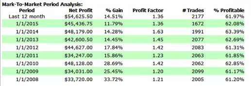
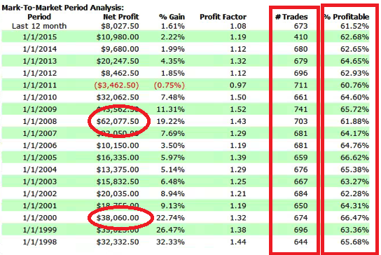
The analysis evaluates the performance of this basic strategy during the “bullish season”, from Nov-May, when the equity markets traditionally make the majority of their annual gains, compared to the outcome during the “bearish season” from Jun-Oct.

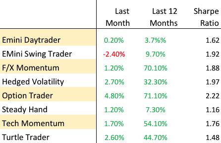
None of the outcomes of these tests is especially noteworthy, save one: the performance during the overnight session in the bullish season:

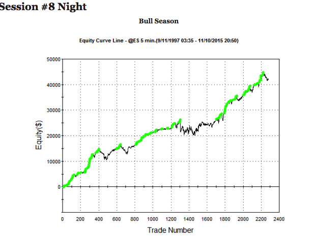
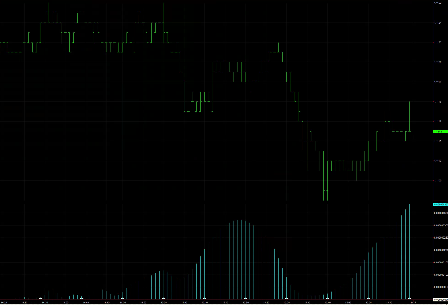
The tendency of the overnight session in the E-mini to produce clearer trends and trading signals has been well documented. Plausible explanations for this phenomenon are that:

(a) The returns process in the overnight session is less contaminated with noise, which primarily results from trading activity; and/or

(b) The relatively poor liquidity of the overnight session allows participants to push the market in one direction more easily.

Either way, there is no denying that this study and several other, similar studies appear to demonstrate interesting trading opportunities in the overnight market.

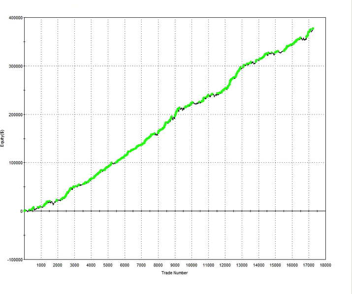
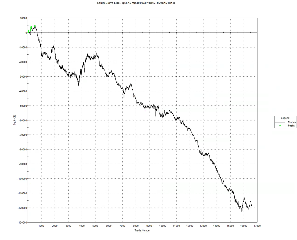
That is, until trading costs are considered. Results for the trading strategy from Nov 1997-Nov 2015 show a gain of $54,575, but an average trade of only just over $20:

Gross PL	# Trades	Av Trade
$54,575	2701	$20.21

Assuming that we enter and exit aggressively, buying at the market at the start of the session and selling MOC at the close, we will pay the bid-offer spread and commissions amounting to around $30, producing a net loss of $10 per trade.

The situation can be improved by omitting January from the “bullish season”, but the slightly higher average trade is still insufficient to overcome trading costs :

Gross PL	# Trades	Av Trade
$54,550	2327	$23.44

Designing a Seasonal Trading Strategy for the Overnight Session

At this point an academic research paper might conclude that the apparently anomalous trading profits are subsumed within the bid-offer spread. But for a trading system designer this is not the end of the story.

If the profits are insufficient to overcome trading frictions when we cross the spread on entry and exit, what about a trading strategy that permits market orders on only the exit leg of the trade, while using limit orders to enter? Total trading costs will be reduced to something closer to $17.50 per round turn, leaving a net profit of almost $6 per trade.

Of course, there is no guarantee that we will successfully enter every trade – our limit orders may not be filled at the bid price and, indeed, we are likely to suffer adverse selection – i.e. getting filled on every losing trading, while missing a proportion of the winning trades.

On the other hand, we are hardly obliged to hold a position for the entire overnight session. Nor are we obliged to exit every trade MOC – we might find opportunities to exit prior to the end of the session, using limit orders to achieve a profit target or cap a trading loss. In such a system, some proportion of the trades will use limit orders on both entry and exit, reducing trading costs for those trades to around $5 per round turn.

The key point is that we can use the seasonal effects detected in the overnight session as a starting point for the development for a more sophisticated trading system that uses a variety of entry and exit criteria, and order types.

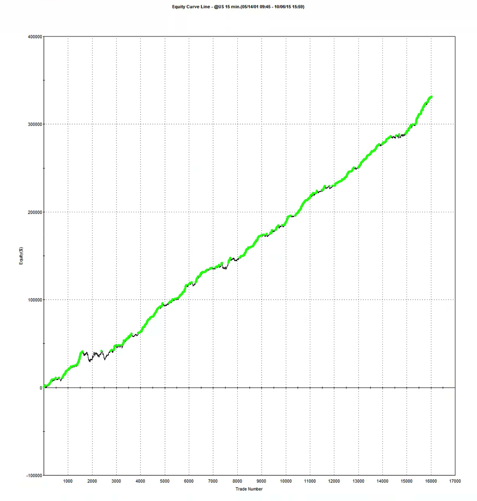
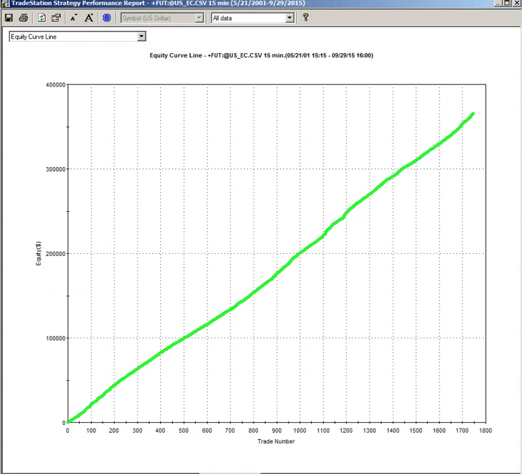
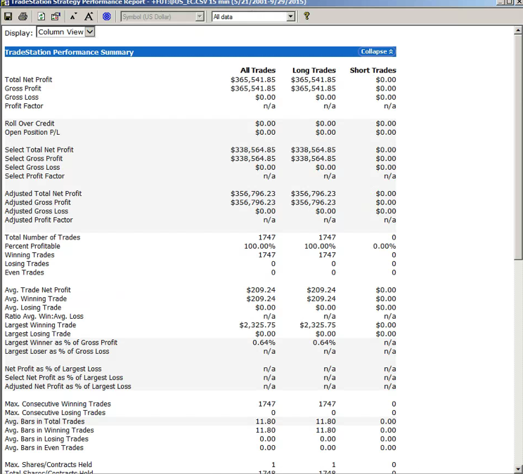
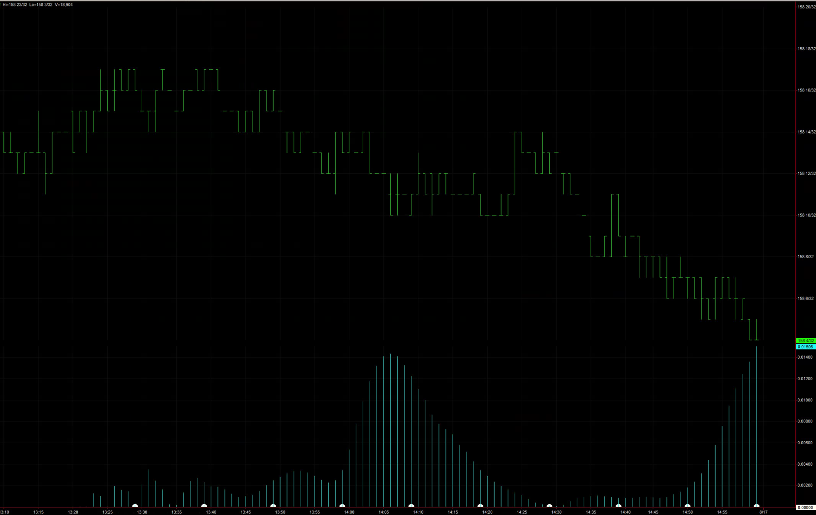
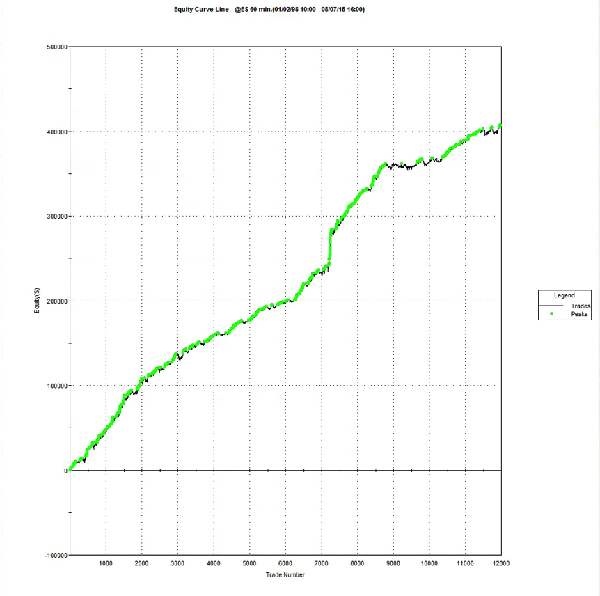
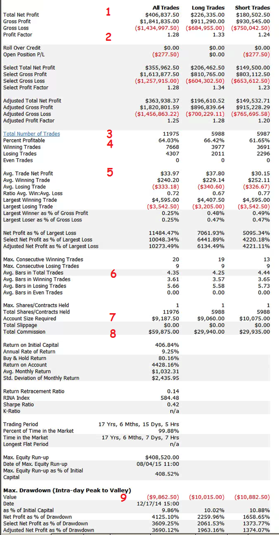
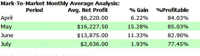
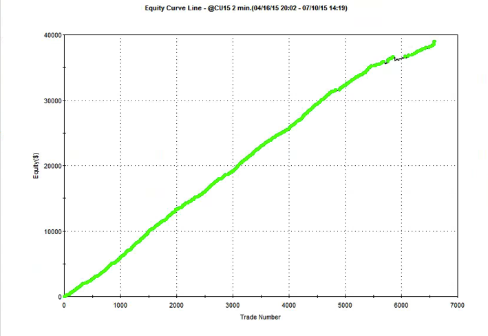
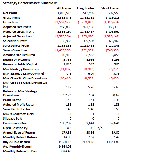
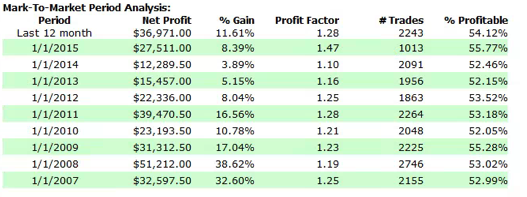
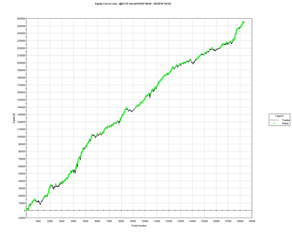
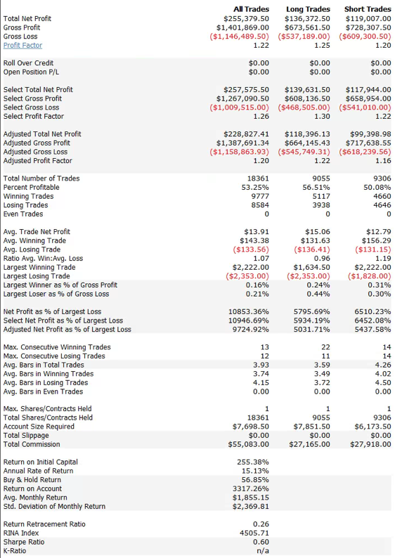
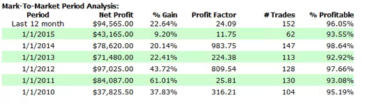
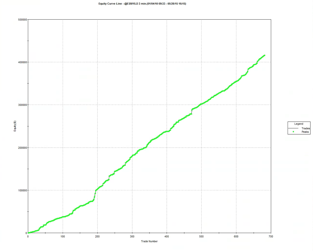
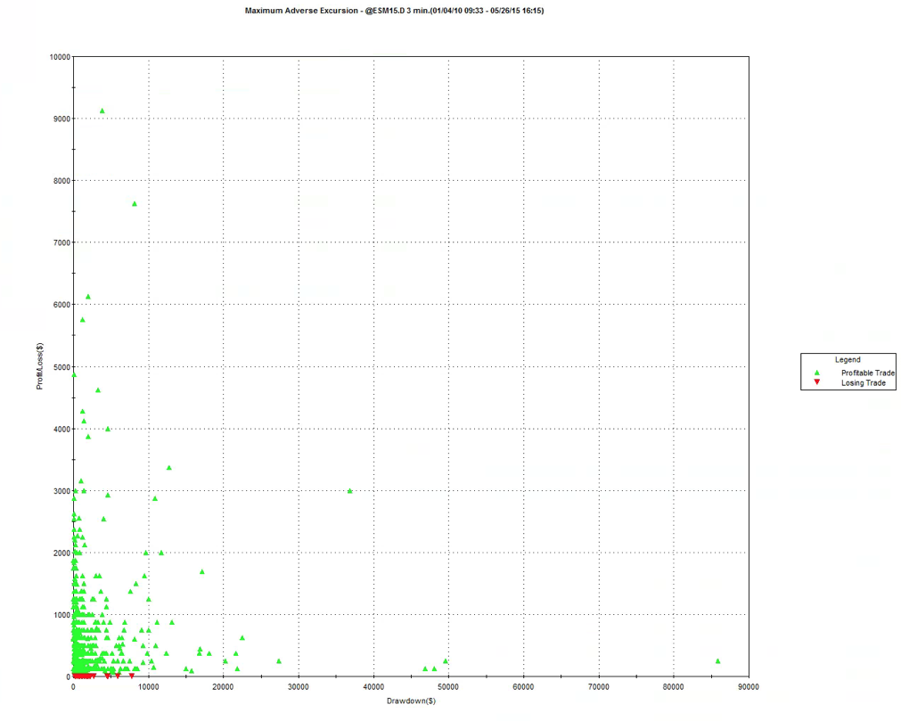
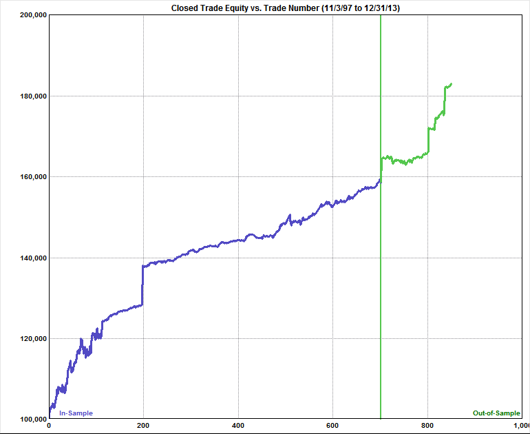
The following shows the performance results for a trading system designed to trade 30-minute bars in the E-mini futures overnight session during the months of Nov to May.The strategy enters trades using limit prices and exits using a combination of profit targets, stop loss targets, and MOC orders.

Data from 1997 to 2010 were used to design the system, which was tested on out-of-sample data from 2011 to 2013. Unseen data from Jan 2014 to Nov 2015 were used to provide a further (double blind) evaluation period for the strategy.

	ALL TRADES	LONG	SHORT
Closed Trade Net Profit	$83,080	$61,493	$21,588
Gross Profit	$158,193	$132,573	$25,620
Gross Loss	-$75,113	-$71,080	-$4,033
Profit Factor	2.11	1.87	6.35
Ratio L/S Net Profit	2.85
Total Net Profit	$83,080	$61,493	$21,588
Trading Period	11/13/97 2:30:00 AM to 12/31/13 6:30:00 AM (16 years 48 days)
Number of Trading Days	2767
Starting Account Equity	$100,000
Highest Equity	$183,080
Lowest Equity	$97,550
Final Closed Trade Equity	$183,080
Return on Starting Equity	83.08%
Number of Closed Trades	849	789	60
Number of Winning Trades	564	528	36
Number of Losing Trades	285	261	24
Trades Not Taken	0	0	0
Percent Profitable	66.43%	66.92%	60.00%
Trades Per Year	52.63	48.91	3.72
Trades Per Month	4.39	4.08	0.31
Max Position Size	1	1	1
Average Trade (Expectation)	$97.86	$77.94	$359.79
Average Trade (%)	0.07%	0.06%	0.33%
Trade Standard Deviation	$641.97	$552.56	$1,330.60
Trade Standard Deviation (%)	0.48%	0.44%	1.20%
Average Bars in Trades	15.2	14.53	24.1
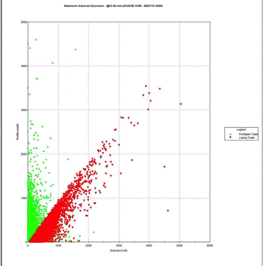
Average MAE	$190.34	$181.83	$302.29
Average MAE (%)	0.14%	0.15%	0.27%
Maximum MAE	$3,237	$2,850	$3,237
Maximum MAE (%)	2.77%	2.52%	3.10%
Win/Loss Ratio	1.06	0.92	4.24
Win/Loss Ratio (%)	2.10	1.83	7.04
Return/Drawdown Ratio	15.36	14.82	5.86
Sharpe Ratio	0.43	0.46	0.52
Sortino Ratio	1.61	1.69	6.40
MAR Ratio	0.71	0.73	0.33
Correlation Coefficient	0.95	0.96	0.719
Statistical Significance	100%	100%	97.78%
Average Risk	$1,099	$1,182	$0.00
Average Risk (%)	0.78%	0.95%	0.00%
Average R-Multiple (Expectancy)	0.0615	0.0662	0
R-Multiple Standard Deviation	0.4357	0.4357	0
Average Leverage	0.399	0.451	0.463
Maximum Leverage	0.685	0.694	0.714
Risk of Ruin	0.00%	0.00%	0.00%
Kelly f	34.89%	31.04%	50.56%
Average Annual Profit/Loss	$5,150	$3,811	$1,338
Ave Annual Compounded Return	3.82%	3.02%	1.22%
Average Monthly Profit/Loss	$429.17	$317.66	$111.52
Ave Monthly Compounded Return	0.31%	0.25%	0.10%
Average Weekly Profit/Loss	$98.70	$73.05	$25.65
Ave Weekly Compounded Return	0.07%	0.06%	0.02%
Average Daily Profit/Loss	$30.03	$22.22	$7.80
Ave Daily Compounded Return	0.02%	0.02%	0.01%
INTRA-BAR EQUITY DRAWDOWNS	ALL TRADES	LONG	SHORT
Number of Drawdowns	445	422	79
Average Drawdown	$282.88	$269.15	$441.23
Average Drawdown (%)	0.21%	0.20%	0.33%
Average Length of Drawdowns	10 days 19 hours	10 days 20 hours	66 days 1 hours
Average Trades in Drawdowns	3	3	1
Worst Case Drawdown	$6,502	$4,987	$4,350
Date at Trough	12/13/00 1:30	5/24/00 4:30	12/13/00 1:30

March 5, 2019

Improving A Hedge Fund Investment – Cantab Capital’s Quantitative Aristarchus Fund

In this post I am going to take a look at what an investor can do to improve a hedge fund investment through the use of dynamic capital allocation. For the purposes of illustration I am going to use Cantab Capital’s Aristarchus program – a quantitative fund which has grown to over $3.5Bn in assets under management since its opening with $30M in 2007 by co-founders Dr. Ewan Kirk and Erich Schlaikjer.

I chose this product because, firstly, it is one of the most successful quantitative funds in existence and, secondly, because as a CTA its performance record is publicly available.

Cantab’s Aristarchus Fund

Cantab’s stated investment philosophy is that algorithmic trading can help to overcome cognitive biases inherent in human-based trading decisions, by exploiting persistent statistical relationships between markets. Taking a multi-asset, multi-model approach, the majority of Cantab’s traded instruments are liquid futures and forwards, across currencies, fixed income, equity indices and commodities.

Let’s take a look at how that has worked out in practice:

Whatever the fund’s attractions may be, we can at least agree that alpha is not amongst them. A Sharpe ratio of < 0.5 (I calculate to be nearer 0.41) is hardly in Renaissance territory, so one imagines that the chief benefit of the product must lie in its liquidity and low market correlation. Uncorrelated it may be, but an investor in the fund must have extremely deep pockets – and a very strong stomach – to handle the 34% drawdown that the fund suffered in 2013.

Improving the Aristarchus Fund Performance

If we make the assumption that an investment in this product is warranted in the first place, what can be done to improve its performance characteristics? We’ll look at that question from two different perspectives – the investor’s and the manager’s.

Firstly, from the investor’s perspective, there are relatively few options available to enhance the fund’s contribution, other than through diversification. One other possibility available to the investor, however, is to develop a program for dynamic capital allocation. This requires the manager to be open to allowing significant changes in the amount of capital to be allocated from month to month, or quarter to quarter, but in a liquid product like Aristarchus some measure of flexibility ought to be feasible.

An analysis of the fund’s performance indicates the presence of a strong dependency in the returns process. This is not at all unusual. Often investment strategies have a tendency to mean-revert: a negative dependency in which periods of poor performance tend to be followed by positive performance, and vice versa. CTA strategies such as Aristarchus tend to be trend-following, and this can induce positive dependency in the strategy returns process, in which positive months tend to follow earlier positive months, while losing months tend to be followed by further losses. This is the pattern we find here.

Consequently, rather than maintaining a constant capital allocation, an investor would do better to allocate capital dynamically, increasing the amount of capital after a positive period, while decreasing the allocation after a period of losses. Let’s consider a variation of this allocation plan, in which the amount of allocated capital is increased by 70% when the last monthly equity value exceeds the quarterly moving average, while the allocation is reduced to zero when the last month’s equity falls below the average. A dynamic capital allocation plan as simple as this appears to produce a significant improvement in the overall performance of the investment:

The slight increase in annual volatility in the returns produced by the dynamic capital allocation model is more than offset by the 412bp improvement in the CAGR. Consequently, the Sharpe Ratio improves from o.41 to 0.60.

Nor is this by any means the entire story: the dynamic model produces lower average drawdowns (7.93% vs. 8.52%) and, more importantly, reduces the maximum drawdown over the life of the fund from a painful 34.87% to more palatable 23.92%.

The much-improved risk profile of the dynamic allocation scheme is reflected in the Return/Drawdown Ratio, which rises from 2.44 to 6.52.

Note, too, that the average level of capital allocated in the dynamic scheme is very slightly less than the original static allocation. In other words, the dynamic allocation technique results in a more efficient use of capital, while at the same time producing a higher rate of risk-adjusted return and enhancing the overall risk characteristics of the strategy.

Improving Fund Performance Using a Meta-Strategy

So much for the investor. What could the manager to do improve the strategy performance? Of course, there is nothing in principle to prevent the manager from also adopting a dynamic approach to capital allocation, although his investment mandate may require him to be fully invested at all times.

Assuming for the moment that this approach is not available to the manager, he can instead look into the possibilities for developing a meta-strategy. As I explained in my earlier post on the topic:

A meta-strategy is a trading system that trades trading systems. The idea is to develop a strategy that will make sensible decisions about when to trade a specific system, in a way that yields superior performance compared to simply following the underlying trading system.

It turns out to be quite straightforward to develop such a meta-strategy, using a combination of stop-loss limits and profit targets to decide when to turn the strategy on or off. In so doing, the manager is able to avoid some periods of negative performance, producing a significant uplift in the overall risk-adjusted return:

Conclusion

Meta-strategies and dynamic capital allocation schemes can enable the investor and the investment manager to improve the performance characteristics of their investment and investment strategy, by increasing returns, reducing volatility and the propensity of the strategy to produce substantial drawdowns.

We have demonstrated how these approaches can be applied successfully to Cantab’s Aristarchus quantitative fund, producing substantial gains in risk adjusted performance and reductions in the average and maximum drawdowns produced over the life of the fund.

January 29, 2019

Improving Trading System Performance Using a Meta-Strategy

What is a Meta-Strategy?

In my previous post on identifying drivers of strategy performance I mentioned the possibility of developing a meta-strategy.

A meta-strategy is a trading system that trades trading systems. The idea is to develop a strategy that will make sensible decisions about when to trade a specific system, in a way that yields superior performance compared to simply following the underlying trading system. Put another way, the simplest kind of meta-strategy is a long-only strategy that takes positions in some underlying trading system. At times, it will follow the underlying system exactly; at other times it is out of the market and ignore the trading system’s recommendations.

More generally, a meta-strategy can determine the size in which one, or several, systems should be traded at any point in time, including periods where the size can be zero (i.e. the system is not currently traded). Typically, a meta-strategy is long-only: in theory there is nothing to stop you developing a meta-strategy that shorts your underlying strategy from time to time, but that is a little counter-intuitive to say the least!

A meta-strategy is something that could be very useful for a fund-of-funds, as a way of deciding how to allocate capital amongst managers.

Caissa Capital operated a meta-strategy in its option arbitrage hedge fund back in the early 2000’s. The meta-strategy (we called it a “model management system”) selected from a half dozen different volatility models to be used for option pricing, depending their performance, as measured by around 30 different criteria. The criteria included both statistical metrics, such as the mean absolute percentage error in the forward volatility forecasts, as well as trading performance criteria such as the moving average of the trade PNL. The model management system probably added 100 – 200 basis points per annum to the performance the underlying strategy, so it was a valuable add-on.

Illustration of a Meta-Strategy in US Bond Futures

To illustrate the concept we will use an underlying system that trades US Bond futures at 15-minute bar intervals. The performance of the system is summarized in the chart and table below.

Strategy performance has been very consistent over the last seven years, in terms of the annual returns, number of trades and % win rate. Can it be improved further?

To assess this possibility we create a new data series comprising the points of the equity curve illustrated above. More specifically, we form a series comprising the open, high, low and close values of the strategy equity, for each trade. We will proceed to treat this as a new data series and apply a range of different modeling techniques to see if we can develop a trading strategy, in exactly the same way as we would if the underlying was a price series for a stock.

It is important to note here that, for the meta-strategy at least, we are working in trade-time, not calendar time. The x-axis will measure the trade number of the underlying strategy, rather than the date of entry (or exit) of the underlying trade. Thus equally spaced points on the x-axis represent different lengths of calendar time, depending on the duration of each trade.

It is necessary to work in trade time rather than calendar time because, unlike a stock, it isn’t possible to trade the underlying strategy whenever we want to – we can only enter or exit the strategy at points in time when it is about to take a trade, by accepting that trade or passing on it (we ignore the other possibility which is sizing the underlying trade, for now).

Another question is what kinds of trading ideas do we want to consider for the meta-strategy? In principle one could incorporate almost any trading concept, including the usual range of technical indictors such as RSI, or Bollinger bands. One can go further an use machine learning techniques, including Neural Networks, Random Forest, or SVM.

In practice, one tends to gravitate towards the simpler kinds of trading algorithm, such as moving averages (or MA crossover techniques), although there is nothing to say that more complex trading rules should not be considered. The development process follows a familiar path: you create a hypothesis, for example, that the equity curve of the underlying bond futures strategy tends to be mean-reverting, and then proceed to test it using various signals – perhaps a moving average, in this case. If the signal results in a potential improvement in the performance of the default meta-strategy (which is to take every trade in the underlying system system), one includes it in the library of signals that may ultimately be combined to create the finished meta-strategy.

As with any strategy development you should follows the usual procedure of separating the trade data to create a set used for in-sample modeling and out-of-sample performance testing.

Following this general procedure I arrived at the following meta-strategy for the bond futures trading system.

The modeling procedure for the meta-strategy has succeeded in eliminating all of the losing trades in the underlying bond futures system, during both in-sample and out-of-sample periods (comprising the most recent 20% of trades).

In general, it is unlikely that one can hope to improve the performance of the underlying strategy quite as much as this, of course. But it may well be possible to eliminate a sufficient proportion of losing trades to reduce the equity curve drawdown and/or increase the overall Sharpe ratio by a significant amount.

A Challenge / Opportunity

If you like the meta-strategy concept, but are unsure how to proceed, I may be able to help.

Send me the data for your existing strategy (see details below) and I will attempt to model a meta-strategy and send you the results. We can together evaluate to what extent I have been successful in improving the performance of the underlying strategy.

Here are the details of what you need to do:

1. You must have an existing, profitable strategy, with sufficient performance history (either real, simulated, or a mixture of the two). I don’t need to know the details of the underlying strategy, or even what it is trading, although it would be helpful to have that information.

2. You must send the complete history of the equity curve of the underlying strategy, in Excel format, with column headings Date, Open, High, Low, Close. Each row represents consecutive trades of the underlying system and the O/H/L/C refers to the value of the equity curve for each trade.

3. The history must comprise at least 500 trades as an absolute minimum and preferably 1000 trades, or more.

4. At this stage I can only consider a single underlying strategy (i.e. a single equity curve)

5. You should not include any software or algorithms of any kind. Nothing proprietary, in other words.

6. I will give preference to strategies that have a (partial) live track record.

As my time is very limited these days I will not be able to deal with any submissions that fail to meet these specifications, or to enter into general discussions about the trading strategy with you.

You can reach me at jkinlay@systematic-strategies.com

January 15, 2019

Signal Processing and Sample Frequency

The Importance of Sample Frequency

Too often we apply a default time horizon for our trading, whether it below (daily, weekly) or higher (hourly, 5 minute) frequency. Sometimes the choice is dictated by practical considerations, such as a desire to avoid overnight risk, or the (lack of0 availability of low-latency execution platform.

But there is an alternative approach to the trade frequency decision that often yields superior results in terms of trading performance. The methodology derives from signal processing and the idea essentially is to use Fourier transforms to help identify the cyclical behavior of the strategy alpha and hence determine the best time-frames for sampling and trading. I wrote about this is a previous blog post, in which I described how to use principal components analysis to investigate the factors driving the returns in various pairs trading strategies. Here I want to take a simpler approach, in which we use Fourier analysis to select suitable sample frequencies. The idea is simply to select sample frequencies where the signal strength appears strongest, in the hope that it will lead to superior performance characteristics in what strategy we are trying to develop.

Signal Decomposition for S&P500 eMini Futures

Let’s take as an example the S&P 500 emini futures contract. The chart below shows the continuous ES futures contract plotted at 1-minute intervals from 1998. At the bottom of the chart I have represented the signal analysis as a bar chart (in blue), with each bar representing the amplitude at each frequency. The white dots on the chart identify frequencies that are spaced 10 minutes apart. It is immediately evident that local maxima in the spectrum occur around 40 mins, 60 mins and 120 mins. So a starting point for our strategy research might be to look at emini data sampled at these frequencies. Incidentally, it is worth pointing out that I have restricted the session times to 7AM – 4PM EST, which is where the bulk of the daily volume and liquidity tend to occur. You may get different results if you include data from the Globex session.

This is all very intuitive and unsurprising: the clearest signals occur at frequencies that most traders typically tend to trade, using hourly data, for example. Any strategy developer is already quite likely to consider these and other common frequencies as part of their regular research process. There are many instances of successful trading strategies built on emini data sampled at 60 minute intervals.

Signal Decomposition for US Bond Futures

Let’s look at a rather more interesting example: US (30 year) Bond futures. Unlike the emini contract, the spectral analysis of the US futures contract indicates that the strongest signal by far occurs at a frequency of around 47 minutes. This is decidedly an unintuitive outcome – I can’t think of any reason why such a strong signal should appear at this cycle length, but, statistically it does.

Does it work? Readers can judge for themselves: below is an example of an equity curve for a strategy on US futures sampled at 47 minute frequency over the period from 2002. The strategy has performed very consistently, producing around $25,000 per contract per year, after commissions and slippage.

Conclusion

While I have had similar success with products as diverse as Corn and VIX futures, the frequency domain approach is by no means a panacea: there are plenty of examples where I have been unable to construct profitable strategies for data sampled at the frequencies with very strong signals. Conversely, I have developed successful strategies using data at frequencies that hardly registered at all on the spectrum, but which I selected for other reasons. Nonetheless, spectral analysis (and signal processing in general) can be recommended as a useful tool in the arsenal of any quantitative analyst.

January 8, 2019

Trading Strategy Design

In this post I want to share some thoughts on how to design great automated trading strategies – what to look for, and what to avoid.

For illustrative purposes I am going to use a strategy I designed for the ever-popular S&P500 e-mini futures contract.

The overall equity curve for the strategy is show below.

This is often the best place to start. What you want to see, of course, is a smooth, upward-sloping curve, without too many sizable drawdowns, and one in which the strategy continues to make new highs. This is especially important in the out-of-sample test period (Jan 2014- Jul 2015 in this case). You will notice a flat period around 2013, which we will need to explore later. Overall, however, this equity curve appears to fit the stereotypical pattern we hope to see when developing a new strategy.

Let’s move on look at the overall strategy performance numbers.

STRATEGY PERFORMANCE CHARACTERISTICS

(click to enlarge)

1. Net Profit
Clearly, the most important consideration. Over the 17 year test period the strategy has produced a net profit averaging around $23,000 per annum, per contract. As a rough guide, you would want to see a net profit per contract around 10x the maintenance margin, or higher.

2. Profit Factor
The gross profit divided by the gross loss. You want this to be as high as possible. Too low, as the strategy will be difficult to trade, because you will see sustained periods of substantial losses. I would suggest a minimum acceptable PF in the region of 1.25. Many strategy developers aim for a PF of 1.5, or higher.

3. Number of Trades
Generally, the more trades the better, at least from the point of view of building confidence in the robustness of strategy performance. A strategy may show a great P&L, but if it only trades once a month it is going to take many many years of performance data to ensure statistical significance. This strategy, on the other hand, is designed to trade 2-3 times a day. Given that, and the length of the test period, there is little doubt that the results are statistically significant.

Profit Factor and number of trades are opposing design criteria – increasing the # trades tends to reduce the PF. That consideration sets an upper bound on the # trades that can be accommodated, before the profit factor deteriorates to unacceptably low levels. Typically, 4-5 trades a day is about the maximum trading frequency one can expect to achieve.

4. Win Rate
Novice system designers tend to assume that you want this to be as high as possible, but that isn’t typically the case. It is perfectly feasible to design systems that have a 90% win rate, or higher, but which produce highly undesirable performance characteristics, such as frequent, large drawdowns. For a typical trading system the optimal range for the win rate is in the region of 40% to 66%. Below this range, it becomes difficult to tolerate the long sequences of losses that will result, without losing faith in the system.

5. Average Trade
This is the average net profit per trade. A typical range would be $10 to $100. Many designers will only consider strategies that have a higher average trade than this one, perhaps $50-$75, or more. The issue with systems that have a very small average trade is that the profits can quickly be eaten up by commissions. Even though, in this case, the results are net of commissions, one can see a significant deterioration in profits if the average trade is low and trade frequency is high, because of the risk of low fill rates (i.e. the % of limit orders that get filled). To assess this risk one looks at the number of fills assumed to take place at the high or low of the bar. If this exceeds 10% of the total # trades, one can expect to see some slippage in the P&L when the strategy is put into production.

6. Average Bars
The number of bars required to complete a trade, on average. There is no hard limit one can suggest here – it depends entirely on the size of the bars. Here we are working in 60 minute bars, so a typical trade is held for around 4.5 hours, on average. That’s a time-frame that I am comfortable with. Others may be prepared to hold positions for much longer – days, or even weeks.

Perhaps more important is the average length of losing trades. What you don’t want to see is the strategy taking far longer to exit losing trades than winning trades. Again, this is a matter of trader psychology – it is hard to sit there hour after hour, or day after day, in a losing position – the temptation to cut the position becomes hard to ignore. But, in doing that you are changing the strategy characteristics in a fundamental way, one that rarely produces a performance improvement.

What the strategy designer needs to do is to figure out in advance what the limits are of the investor’s tolerance for pain, in terms of maximum drawdown, average losing trade, etc, and design the strategy to meet those specifications, rather than trying to fix the strategy afterwards.

7. Required Account Size
It’s good to know exactly how large an account you need per contract, so you can figure out how to scale the strategy. In this case one could hope to scale the strategy up to a 10-lot in a $100,000 account. That may or may not fit the trader’s requirements and again, this needs to be considered at the outset. For example, for a trader looking to utilize, say, $1,000,000 of capital, it is doubtful whether this strategy would fit his requirements without considerable work on the implementations issues that arise when trying to trade in anything approaching a 100 contract clip rate.

8. Commission
Always check to ensure that the strategy designer has made reasonable assumptions about slippage and commission. Here we are assuming $5 per round turn. There is no slippage, because the strategy executes using limit orders.

9. Drawdown
Drawdowns are, of course, every investor’s bugbear. No-one likes drawdowns that are either large, or lengthy in relation to the annual profitability of the strategy, or the average trade duration. A $10,000 max drawdown on a strategy producing over $23,000 a year is actually quite decent – I have seen many e-mini strategies with drawdowns at 2x – 3x that level, or larger. Again, this is one of the key criteria that needs to be baked into the strategy design at the outset, rather than trying to fix later.

ANNUAL PROFITABILITY

Let’s now take a look at how the strategy performs year-by-year, and some of the considerations and concerns that often arise.

1. Performance During Downturns
One aspect I always pay attention to is how well the strategy performs during periods of high market stress, because I expect similar conditions to arise in the fairly near future, e.g. as the Fed begins to raise rates.

Here, as you can see, the strategy performed admirably during both the dot com bust of 1999/2000 and the financial crisis of 2008/09.

2. Consistency in the # Trades and % Win Rate
It is not uncommon with low frequency strategies to see periods of substantial variation in the # trades or win rate. Regardless how good the overall performance statistics are, this makes me uncomfortable. It could be, for instance, that the overall results are influenced by one or two exceptional years that are unlikely to be repeated. Significant variation in the trading or win rate raise questions about the robustness of the strategy, going forward. On the other hand, as here, it is a comfort to see the strategy maintaining a very steady trading rate and % win rate, year after year.

3. Down Years
Every strategy shows variation in year to year performance and one expects to see years in which the strategy performs less well, or even loses money. For me, it rather depends on when such losses arise, as much as the size of the loss. If a loss occurs in the out-of-sample period it raises serious questions about strategy robustness and, as a result, I am very unlikely to want to put such a strategy into production. If, as here, the period of poor performance occurs during the in-sample period I am less concerned – the strategy has other, favorable characteristics that make it attractive and I am willing to tolerate the risk of one modestly down-year in over 17 years of testing.

INTRA-TRADE DRAWDOWNS

Many trades that end up being profitable go through a period of being under-water. What matters here is how high those intra-trade losses may climb, before the trade is closed. To take an extreme example, would you be willing to risk $10,000 to make an average profit of only $10 per trade? How about $20,000? $50,000? Your entire equity?

The Maximum Average Excursion chart below shows the drawdowns on a trade by trade basis. Here we can see that, over the 17 year test period, no trade has suffered a drawdown of much more than $5,000. I am comfortable with that level. Others may prefer a lower limit, or be tolerant of a higher MAE.

Again, the point is that the problem of a too-high MAE is not something one can fix after the event. Sure, a stop loss will prevent any losses above a specified size. But a stop loss also has the unwanted effect of terminating trades that would have turned into money-makers. While psychologically comfortable, the effect of a stop loss is almost always negative in terms of strategy profitability and other performance characteristics, including drawdown, the very thing that investors are looking to control.

CONCLUSION
I have tried to give some general guidelines for factors that are of critical importance in strategy design. There are, of course, no absolutes: the “right” characteristics depend entirely on the risk preferences of the investor.

One point that strategy designers do need to take on board is the need to factor in all of the important design criteria at the outset, rather than trying (and usually failing) to repair the strategy shortcomings after the event.

December 25, 2018

Making Money with High Frequency Trading

There is no standard definition of high frequency trading, nor a single type of strategy associated with it. Some strategies generate returns, not by taking any kind of view on market direction, but simply by earning Exchange rebates. In other cases the strategy might try to trade ahead of the news as it flows through the market, from stock to stock (or market to market). Perhaps the most common and successful approach to HFT is market making, where one tries to earn (some fraction of) the spread by constantly quoting both sides of the market. In the latter approach, which involves processing vast numbers of order messages and other market data in order to decide whether to quote (or pull a quote), latency is of utmost importance. I would tend to argue that HFT market making owes its success as much, or more, to computer science than it does to trading or microstructure theory.

By contrast, Systematic Strategies’s approach to HFT has always been model-driven. We are unable to outgun firms like Citadel or Getco in terms of their speed of execution; so, instead, we focus on developing theoretical models of market behavior, on the assumption that we are more likely to identify a source of true competitive advantage that way. This leads to slower, less latency-sensitive strategies (the models have to be re-estimated or recomputed in real time), but which may nonetheless trade hundreds of times a day.

A good example is provided by our high frequency scalping strategy in Corn futures, which trades around 100-200 times a day, with a win rate of over 80%.

One of the most important considerations in engineering a HFT strategy of this kind is to identify a suitable bar frequency. We find that our approach works best using data at frequencies of 1-5 minutes, trading at latencies of around 1 millisec, whereas other firms are reacting to data tick-by-tick, with latencies measured in microseconds.

Often strategies are built using only data derived from with a single market, based on indicators involving price action, pattern trading rules, volume or volatility signals. In other cases, however, signals are derived from other, related markets: the VXX-ES-TY complex would be a typical example of this kind of inter-market approach.

When we build strategies we often start by using a simple retail platform like TradeStation or MultiCharts. We know that if the strategy can make money on a platform with retail levels of order and market data latency (and commission rates), then it should perform well when we transfer it to a production environment, with much lower latencies and costs. We might be able to trade only 1-2 contracts in TradeStation, but in production we might aim to scale that up to 10-15 contract per trade, or more, depending on liquidity. For that reason we prefer to trade only intraday, when market liquidity is deepest; but we often find sufficient levels of liquidity to make trading worthwhile 1-2 hours before the open of the day session.

Generally, while we look for outside money for our lower frequency hedge fund strategies, we tend not to do so for our HFT strategies. After all, what’s the point? Each strategy has limited capacity and typically requires no more than a $100,000 account, at most. And besides, with Sharpe Ratios that are typically in double-digits, it’s usually in our economic interest to use all of the capacity ourselves. Nor do we tend to license strategies to other trading firms. Again, why would we? If the strategies work, we can earn far more from trading rather than licensing them.

We have, occasionally, developed strategies for other firms for markets in which we have no interest (the KOSPI springs to mind). But these cases tend to be the exception, rather than the rule.

December 4, 2018

High Frequency Trading Strategies

Most investors have probably never seen the P&L of a high frequency trading strategy. There is a reason for that, of course: given the typical performance characteristics of a HFT strategy, a trading firm has little need for outside capital. Besides, HFT strategies can be capacity constrained, a major consideration for institutional investors. So it is amusing to see the reaction of an investor on encountering the track record of a HFT strategy for the first time. Accustomed as they are to seeing Sharpe ratios in the range of 0.5-1.5, or perhaps as high as 1.8, if they are lucky, the staggering risk-adjusted returns of a HFT strategy, which often have double-digit Sharpe ratios, are truly mind-boggling.

By way of illustration I have attached below the performance record of one such HFT strategy, which trades around 100 times a day in the eMini S&P 500 contract (including the overnight session). Note that the edge is not that great – averaging 55% profitable trades and profit per contract of around half a tick – these are some of the defining characteristics of HFT trading strategies. But due to the large number of trades it results in very substantial profits. At this frequency, trading commissions are very low, typically under $0.1 per contract, compared to $1 – $2 per contract for a retail trader (in fact an HFT firm would typically own or lease exchange seats to minimize such costs).

Hidden from view in the above analysis are the overhead costs associated with implementing such a strategy: the market data feed, execution platform and connectivity capable of handling huge volumes of messages, as well as algo logic to monitor microstructure signals and manage order-book priority. Without these, the strategy would be impossible to implement profitably.

Scaling things back a little, lets take a look at a day-trading strategy that trades only around 10 times a day, on 15-minute bars. Although not ultra-high frequency, the strategy nonetheless is sufficiently high frequency to be very latency sensitive. In other words, you would not want to try to implement such a strategy without a high quality market data feed and low-latency trading platform capable of executing at the 1-millisecond level. It might just be possible to implement a strategy of this kind using TT’s ADL platform, for example.

While the win rate and profit factor are similar to the first strategy, the lower trade frequency allows for a higher trade PL of just over 1 tick, while the equity curve is a lot less smooth reflecting a Sharpe ratio that is “only” around 2.7.

The critical assumption in any HFT strategy is the fill rate. HFT strategies execute using limit or IOC orders and only a certain percentage of these will ever be filled. Assuming there is alpha in the signal, the P&L grows in direct proportion to the number of trades, which in turn depends on the fill rate. A fill rate of 10% to 20% is usually enough to guarantee profitability (depending on the quality of the signal). A low fill rate, such as would typically be seen if one attempted to trade on a retail trading platform, would destroy the profitability of any HFT strategy.

To illustrate this point, we can take a look at the outcome if the above strategy was implemented on a trading platform which resulted in orders being filled only when the market trades through the limit price. It isn’t a pretty sight.

The moral of the story is: developing a HFT trading algorithm that contains a viable alpha signal is only half the picture. The trading infrastructure used to implement such a strategy is no less critical. Which is why HFT firms spend tens, or hundreds of millions of dollars developing the best infrastructure they can afford.

November 27, 2018

Designing a Scalable Futures Strategy

I have been working on a higher frequency version of the eMini S&P 500 futures strategy, based on 3-minute bar intervals, which is designed to trade a couple of times a week, with hold periods of 2-3 days. Even higher frequency strategies are possible, of course, but my estimation is that a hold period of under a week provides the best combination of liquidity and capacity. Furthermore, the strategy is of low enough frequency that it is not at all latency sensitive – indeed, in the performance analysis below I have assumed that the market must trade through the limit price before the system enters a trade (relaxing the assumption and allowing the system to trade when the market touches the limit price improves the performance).

The other important design criteria are the high % of profitable trades and Kelly f (both over 95%). This enables the investor to employ money management techniques, such a fixed-fractional allocation for example, in order to scale the trade size up from 1 to 10 contracts, without too great a risk of a major drawdown in realized P&L.

The end result is a strategy that produces profits of $80,000 to $100,000 a year on a 10 contract position, with an annual rate of return of 30% and a Sharpe ratio in excess of 2.0.

Furthermore, of the 682 trades since Jan 2010, only 29 have been losers.

Annual P&L (out of sample)

Equity Curve

Strategy Performance

What’s the Downside?

Everything comes at a price, of course. Firstly, the strategy is long-only and, by definition, will perform poorly in falling markets, such as we saw in 2008. That’s a defensible investment thesis, of course – how many $billions are invested in buy and hold strategies? – and, besides, as one commentator remarked, the trick is to develop multiple strategies for different market regimes (although, sensible as that sounds, one is left with the difficulty of correctly identifying the market regime).

The second drawback is revealed by the trade chart below, which plots the drawdown experienced during each trade. The great majority of these drawdowns are unrealized, and in most cases the trade recovers to make a profit. However, there are some very severe cases, such as Sept 2014, when the strategy experienced a drawdown of $85,000 before recovering to make a profit on the trade. For most investors, the agony of risking an entire year’s P&L just to make a few hundred dollars would be too great.

It should be pointed out that the by the time the drawdown event took place the strategy had already produced many hundreds of thousands of dollars of profit. So, one could take the view that by that stage the strategy was playing with “house money” and could well afford to take such a risk.

One obvious “solution” to the drawdown problem is to use some kind of stop loss. Unfortunately, the effect is simply to convert an unrealized drawdown into a realized loss. For some, however, it might be preferable to take a hit of $40,000 or $50,000 once every few years, rather than suffer the uncertainty of an even larger potential loss. Either way, despite its many pleasant characteristics, this is not a strategy for investors with weak stomachs!

October 2, 2018October 2, 2018

Quant Strategies in 2018

Quant Strategies – Performance Summary Sept. 2018

The end of Q3 seems like an appropriate time for an across-the-piste review of how systematic strategies are performing in 2018. I’m using the dozen or more strategies running on the Systematic Algotrading Platform as the basis for the performance review, although results will obviously vary according to the specifics of the strategy. All of the strategies are traded live and performance results are net of subscription fees, as well as slippage and brokerage commissions.

Volatility Strategies

Those waiting for the hammer to fall on option premium collecting strategies will have been disappointed with the way things have turned out so far in 2018. Yes, February saw a long-awaited and rather spectacular explosion in volatility which completely destroyed several major volatility funds, including the VelocityShares Daily Inverse VIX Short-Term ETN (XIV) as well as Chicago-based hedged fund LJM Partners (“our goal is to preserve as much capital as possible”), that got caught on the wrong side of the popular VIX carry trade. But the lack of follow-through has given many volatility strategies time to recover. Indeed, some are positively thriving now that elevated levels in the VIX have finally lifted option premiums from the bargain basement levels they were languishing at prior to February’s carnage. The Option Trader strategy is a stand-out in this regard: not only did the strategy produce exceptional returns during the February melt-down (+27.1%), the strategy has continued to outperform as the year has progressed and YTD returns now total a little over 69%. Nor is the strategy itself exceptionally volatility: the Sharpe ratio has remained consistently above 2 over several years.

Hedged Volatility Trading

Investors’ chief concern with strategies that rely on collecting option premiums is that eventually they may blow up. For those looking for a more nuanced approach to managing tail risk the Hedged Volatility strategy may be the way to go. Like many strategies in the volatility space the strategy looks to generate alpha by trading VIX ETF products; but unlike the great majority of competitor offerings, this strategy also uses ETF options to hedge tail risk exposure. While hedging costs certainly acts as a performance drag, the results over the last few years have been compelling: a CAGR of 52% with a Sharpe Ratio close to 2.

F/X Strategies

One of the common concerns for investors is how to diversify their investment portfolios, especially since the great majority of assets (and strategies) tend to exhibit significant positive correlation to equity indices these days. One of the characteristics we most appreciate about F/X strategies in general and the F/X Momentum strategy in particular is that its correlation to the equity markets over the last several years has been negligible. Other attractive features of the strategy include the exceptionally high win rate – over 90% – and the profit factor of 5.4, which makes life very comfortable for investors. After a moderate performance in 2017, the strategy has rebounded this year and is up 56% YTD, with a CAGR of 64.5% and Sharpe Ratio of 1.89.

Equity Long/Short

Thanks to the Fed’s accommodative stance, equity markets have been generally benign over the last decade to the benefit of most equity long-only and long-short strategies, including our equity long/short Turtle Trader strategy , which is up 31% YTD. This follows a spectacular 2017 (+66%) , and is in line with the 5-year CAGR of 39%. Notably, the correlation with the benchmark S&P500 Index is relatively low (0.16), while the Sharpe Ratio is a respectable 1.47.

Equity ETFs – Market Timing/Swing Trading

One alternative to the traditional equity long/short products is the Tech Momentum strategy. This is a swing trading strategy that exploits short term momentum signals to trade the ProShares UltraPro QQQ (TQQQ) and ProShares UltraPro Short QQQ (SQQQ) leveraged ETFs. The strategy is enjoying a banner year, up 57% YTD, with a four-year CAGR of 47.7% and Sharpe Ratio of 1.77. A standout feature of this equity strategy is its almost zero correlation with the S&P 500 Index. It is worth noting that this strategy also performed very well during the market decline in Feb, recording a gain of over 11% for the month.

Futures Strategies

It’s a little early to assess the performance of the various futures strategies in the Systematic Strategies portfolio, which were launched on the platform only a few months ago (despite being traded live for far longer). For what it is worth, both of the S&P 500 E-Mini strategies, the Daytrader and the Swing Trader, are now firmly in positive territory for 2018. Obviously we are keeping a watchful eye to see if the performance going forward remains in line with past results, but our experience of trading these strategies gives us cause for optimism.

Conclusion: Quant Strategies in 2018

There appear to be ample opportunities for investors in the quant sector across a wide range of asset classes. For investors with equity market exposure, we particularly like strategies with low market correlation that offer significant diversification benefits, such as the F/X Momentum and F/X Momentum strategies. For those investors seeking the highest risk adjusted return, option selling strategies like the Option Trader strategy are the best choice, while for more cautious investors concerned about tail risk the Hedged Volatility strategy offers the security of downside protection. Finally, there are several new strategies in equities and futures coming down the pike, several of which are already showing considerable promise. We will review the performance of these newer strategies at the end of the year.

Go here for more information about the Systematic Algotrading Platform.

September 23, 2018

Money Management – the Good, the Bad and the Ugly

The infatuation of futures traders with the subject of money management, (more aptly described as position sizing), is something of a puzzle for someone coming from a background in equities or forex. The idea is, simply, that one can improve one’s trading performance through the judicious use of leverage, increasing the size of a position at times and reducing it at others.

Perhaps the most widely known money management technique is the Martingale, where the size of the trade is doubled after every loss. It is easy to show mathematically that such a system must win eventually, provided that the bet size is unlimited. It is also easy to show that, small as it may be, there is a non-zero probability of a long string of losing trades that would bankrupt the trader before he was able to recoup all his losses. Still, the prospect offered by the Martingale strategy is an alluring one: the idea that, no matter what the underlying trading strategy, one can eventually be certain of winning. And so a virtual cottage industry of money management techniques has evolved.

One of the reasons why the money management concept is prevalent in the futures industry compared to, say, equities or f/x, is simply the trading mechanics. Doubling the size of a position in futures might mean trading an extra contract, or perhaps a ten-lot; doing the same in equities might mean scaling into and out of multiple positions comprising many thousands of shares. The execution risk and cost of trying to implement a money management program in equities has historically made the idea infeasible, although that is less true today, given the decline in commission rates and the arrival of smart execution algorithms. Still, money management is a concept that originated in the futures industry and will forever be associated with it.

Van Tharp on Position Sizing
I was recently recommended to read Van Tharp’s Definitive Guide to Position Sizing, which devotes several hundred pages to the subject. Leaving aside the great number of pages of simulation results, there is much to commend it. Van Tharp does a pretty good job of demolishing highly speculative and very dangerous “money management” techniques such as the Kelly Criterion and Ralph Vince’s Optimal f, which make unrealistic assumptions of one kind or another, such as, for example, that there are only two outcomes, rather than the multiple possibilities from a trading strategy, or considering only the outcome of a single trade, rather than a succession of trades (whose outcome may not be independent). Just as with the Martingale, these techniques will often produce unacceptably large drawdowns. In fact, as I have pointed out elsewhere, the use of leverage which many so-called money management techniques actually calls for increases in the risk in the original strategy, often reducing its risk-adjusted return.

As Van Tharp points out, mathematical literacy is not one of the strongest suits of futures traders in general and the money management strategy industry reflects that.

But Van Tharp himself is not immune to misunderstanding mathematical concepts. His central idea is that trading systems should be rated according to its System Quality Number, which he defines as:

SQN = (Expectancy / standard deviation of R) * square root of Number of Trades

R is a central concept of Van Tharp’s methodology, which he defines as how much you will lose per unit of your investment. So, for example, if you buy a stock today for $50 and plan to sell it if it reaches $40, your R is $10. In cases like this you have a clear definition of your R. But what if you don’t? Van Tharp sensibly recommends you use your average loss as an estimate of R.

Expectancy, as Van Tharp defines it, is just the expected profit per trade of the system expressed as a multiple of R. So

SQN = ( (Average Profit per Trade / R) / standard deviation (Average Profit per Trade / R) * square root of Number of Trades

Squaring both sides of the equation, we get:

SQN^2 = ( (Average Profit per Trade )^2 / R^2) / Variance (Average Profit per Trade / R) ) * Number of Trades

The R-squared terms cancel out, leaving the following:

SQN^2 = ((Average Profit per Trade ) ^ 2 / Variance (Average Profit per Trade)) * Number of Trades

Hence,

SQN = (Average Profit per Trade / Standard Deviation (Average Profit per Trade)) * square root of Number of Trades

There is another name by which this measure is more widely known in the investment community: the Sharpe Ratio.

On the “Optimal” Position Sizing Strategy
In my view, Van Tharp’s singular achievement has been to spawn a cottage industry out of restating a fact already widely known amongst investment professionals, i.e. that one should seek out strategies that maximize the Sharpe Ratio.

Not that seeking to maximize the Sharpe Ratio is a bad idea – far from it. But then Van Tharp goes on to suggest that one should consider only strategies with a SQN of greater than 2, ideally much higher (he mentions SQNs of the order of 3-6).

But 95% or more of investable strategies have a Sharpe Ratio less than 2. In fact, in the world of investment management a Sharpe Ratio of 1.5 is considered very good. Barely a handful of funds have demonstrated an ability to maintain a Sharpe Ratio of greater than 2 over a sustained period (Jim Simon’s Renaissance Technologies being one of them). Only in the world of high frequency trading do strategies typically attain the kind of Sharpe Ratio (or SQN) that Van Tharp advocates. So while Van Tharp’s intentions are well meaning, his prescription is unrealistic, for the majority of investors.

One recommendation of Van Tharp’s that should be taken seriously is that there is no single “best” money management strategy that suits every investor. Instead, position sizing should be evolved through simulation, taking into account each trader or investor’s preferences in terms of risk and return. This makes complete sense: a trader looking to make 100% a year and willing to risk 50% of his capital is going to adopt a very different approach to money management, compared to an investor who will be satisfied with a 10% return, provided his risk of losing money is very low. Again, however, there is nothing new here: the problem of optimal allocation based on an investor’s aversion to risk has been thoroughly addressed in the literature for at least the last 50 years.

What about the Equity Curve Money Management strategy I discussed in a previous post? Isn’t that a kind of Martingale? Yes and no. Indeed, the strategy does require us to increase the original investment after a period of loss. But it does so, not after a single losing trade, but after a series of losses from which the strategy is showing evidence of recovering. Furthermore, the ECMM system caps the add-on investment at some specified level, rather than continuing to double the trade size after every loss, as in a Martingale.

But the critical difference between the ECMM and the standard Martingale lies in the assumptions about dependency in the returns of the underlying strategy. In the traditional Martingale, profits and losses are independent from one trade to the next. By contrast, scenarios where ECMM is likely to prove effective are ones where there is dependency in the underlying strategy, more specifically, negative autocorrelation in returns over some horizon. What that means is that periods of losses or lower returns tend to be followed by periods of gains, or higher returns. In other words, ECMM works when the underlying strategy has a tendency towards mean reversion.

CONCLUSION
The futures industry has spawned a myriad of position sizing strategies. Many are impractical, or positively dangerous, leading as they do to significant risk of catastrophic loss. Generally, investors should seek out strategies with higher Sharpe Ratios, and use money management techniques only to improve the risk-adjusted return. But there is no universal money management methodology that will suit every investor. Instead, money management should be conditioned on each individual investors risk preferences.