QUANTITATIVE RESEARCH AND TRADING

November 27, 2018

Designing a Scalable Futures Strategy

I have been working on a higher frequency version of the eMini S&P 500 futures strategy, based on 3-minute bar intervals, which is designed to trade a couple of times a week, with hold periods of 2-3 days. Even higher frequency strategies are possible, of course, but my estimation is that a hold period of under a week provides the best combination of liquidity and capacity. Furthermore, the strategy is of low enough frequency that it is not at all latency sensitive – indeed, in the performance analysis below I have assumed that the market must trade through the limit price before the system enters a trade (relaxing the assumption and allowing the system to trade when the market touches the limit price improves the performance).

The other important design criteria are the high % of profitable trades and Kelly f (both over 95%). This enables the investor to employ money management techniques, such a fixed-fractional allocation for example, in order to scale the trade size up from 1 to 10 contracts, without too great a risk of a major drawdown in realized P&L.

The end result is a strategy that produces profits of $80,000 to $100,000 a year on a 10 contract position, with an annual rate of return of 30% and a Sharpe ratio in excess of 2.0.

Furthermore, of the 682 trades since Jan 2010, only 29 have been losers.

Annual P&L (out of sample)

Equity Curve

Strategy Performance

What’s the Downside?

Everything comes at a price, of course. Firstly, the strategy is long-only and, by definition, will perform poorly in falling markets, such as we saw in 2008. That’s a defensible investment thesis, of course – how many $billions are invested in buy and hold strategies? – and, besides, as one commentator remarked, the trick is to develop multiple strategies for different market regimes (although, sensible as that sounds, one is left with the difficulty of correctly identifying the market regime).

The second drawback is revealed by the trade chart below, which plots the drawdown experienced during each trade. The great majority of these drawdowns are unrealized, and in most cases the trade recovers to make a profit. However, there are some very severe cases, such as Sept 2014, when the strategy experienced a drawdown of $85,000 before recovering to make a profit on the trade. For most investors, the agony of risking an entire year’s P&L just to make a few hundred dollars would be too great.

It should be pointed out that the by the time the drawdown event took place the strategy had already produced many hundreds of thousands of dollars of profit. So, one could take the view that by that stage the strategy was playing with “house money” and could well afford to take such a risk.

One obvious “solution” to the drawdown problem is to use some kind of stop loss. Unfortunately, the effect is simply to convert an unrealized drawdown into a realized loss. For some, however, it might be preferable to take a hit of $40,000 or $50,000 once every few years, rather than suffer the uncertainty of an even larger potential loss. Either way, despite its many pleasant characteristics, this is not a strategy for investors with weak stomachs!

November 20, 2018

Investing in Leveraged ETFs – Theory and Practice

Summary

Leveraged ETFs suffer from decay, or “beta slippage.” Researchers have attempted to exploit this effect by shorting pairs of long and inverse leveraged ETFs.

The results of these strategies look good if you assume continuous compounding, but are often poor when less frequent compounding is assumed.

In reality, the trading losses incurred in rebalancing the portfolio, which requires you to sell low and buy high, overwhelm any benefit from decay, making the strategies unprofitable in practice.

A short levered ETF strategy has similar characteristics to a short straddle option position, with positive Theta and negative Gamma, and will experience periodic, large drawdowns.

It is possible to develop leveraged ETF strategies producing high returns and Sharpe ratios with relative value techniques commonly used in option trading strategies.

Decay in Leveraged ETFs

Leveraged ETFs continue to be much discussed on Seeking Alpha.

One aspect in particular that has caught analysts’ attention is the decay, or “beta slippage” that leveraged ETFs tend to suffer from.

Seeking Alpha contributor Fred Picard in a 2013 article (“What You Need To Know About The Decay Of Leveraged ETFs“) described the effect using the following hypothetical example:

To understand what is beta-slippage, imagine a very volatile asset that goes up 25% one day and down 20% the day after. A perfect double leveraged ETF goes up 50% the first day and down 40% the second day. On the close of the second day, the underlying asset is back to its initial price:

(1 + 0.25) x (1 – 0.2) = 1

And the perfect leveraged ETF?

(1 + 0.5) x (1 – 0.4) = 0.9

Nothing has changed for the underlying asset, and 10% of your money has disappeared. Beta-slippage is not a scam. It is the normal mathematical behavior of a leveraged and rebalanced portfolio. In case you manage a leveraged portfolio and rebalance it on a regular basis, you create your own beta-slippage. The previous example is simple, but beta-slippage is not simple. It cannot be calculated from statistical parameters. It depends on a specific sequence of gains and losses.

Fred goes on to make the point that is the crux of this article, as follows:

At this point, I’m sure that some smart readers have seen an opportunity: if we lose money on the long side, we make a profit on the short side, right?

Shorting Leveraged ETFs

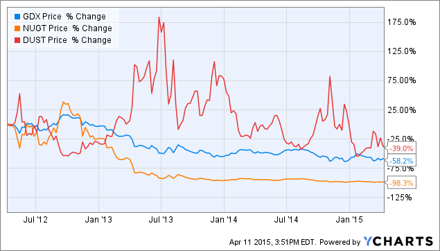
Taking his cue from Fred’s article, Seeking Alpha contributor Stanford Chemist (“Shorting Leveraged ETF Pairs: Easier Said Than Done“) considers the outcome of shorting pairs of leveraged ETFs, including the Market Vectors Gold Miners ETF (NYSEARCA:GDX), the Direxion Daily Gold Miners Bull 3X Shares ETF (NYSEARCA:NUGT) and the Direxion Daily Gold Miners Bear 3X Shares ETF (NYSEARCA:DUST).

His initial finding appears promising:

Therefore, investing $10,000 each into short positions of NUGT and DUST would have generated a profit of $9,830 for NUGT, and $3,900 for DUST, good for an average profit of 68.7% over 3 years, or 22.9% annualized.

At first sight, this appears to a nearly risk-free strategy; after all, you are shorting both the 3X leveraged bull and 3X leveraged bear funds, which should result in a market neutral position. Is there easy money to be made?

Source: Standford Chemist

Not so fast! Stanford Chemist applies the same strategy to another ETF pair, with a very different outcome:

“What if you had instead invested $10,000 each into short positions of the Direxion Russell 1000 Financials Bullish 3X ETF (NYSEARCA:FAS) and the Direxion Russell 1000 Financials Bearish 3X ETF (NYSEARCA:FAZ)?

The $10,000 short position in FAZ would have gained you $8,680. However, this would have been dwarfed by the $28,350 loss that you would have sustained in shorting FAS. In total, you would be down $19,670, which translates into a loss of 196.7% over three years, or 65.6% annualized.

No free lunch there.

The Rebalancing Issue

Stanford Chemist puts his finger on one of the key issues: rebalancing. He explains as follows:

So what happened to the FAS-FAZ pair? Essentially, what transpired was that as the underlying asset XLF increased in value, the two short positions became unbalanced. The losing side (short FAS) ballooned in size, making further losses more severe. On the other hand, the winning side (short FAZ) shrunk, muting the effect of further gains.

To counteract this effect, the portfolio needs to be rebalanced. Stanford Chemist looks at the implications of rebalancing a short NUGT-DUST portfolio whenever the market value of either ETF deviates by more than N% from its average value, where he considers N% in the range from 10% to 100%, in increments of 10%.

While the annual portfolio return was positive in all but one of these scenarios, there was very considerable variation in the outcomes, with several of the rebalanced portfolios suffering very large drawdowns of as much as 75%:

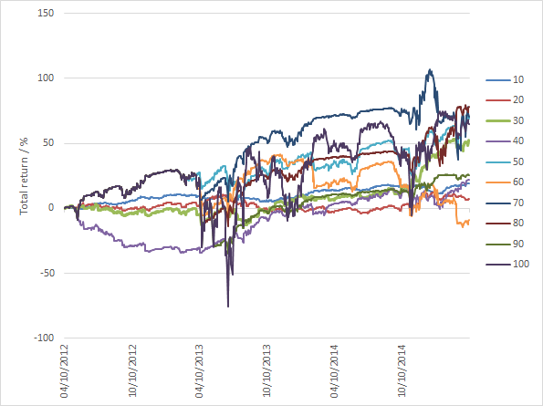
Source: Stanford Chemist

The author concludes:

The results of the backtest showed that profiting from this strategy is easier said than done. The total return performances of the strategy over the past three years was highly dependent on the rebalancing thresholds chosen. Unfortunately, there was also no clear correlation between the rebalancing period used and the total return performance. Moreover, the total return profiles showed that large drawdowns do occur, meaning that despite being ostensibly “market neutral”, this strategy still bears a significant amount of risk.

Leveraged ETF Pairs – Four Case Studies

Let’s press pause here and review a little financial theory. As you recall, it is possible to express a rate of return in many different ways, depending on how interest is compounded. The most typical case is daily compounding:

R = (P_t – P_t-1) / P_t

Where Pt is the price on day t, and P_t-1 is the price on day t-1, one day prior.

Another commonly used alternative is continuous compounding, also sometimes called log-returns:

R = Ln(P_t) – Ln(P_t-1)

Where Ln(P_t) is the natural log of the price on day t, P_t

When a writer refers to a rate of return, he should make clear what compounding basis the return rate is quoted on, whether continuous, daily, monthly or some other frequency. Usually, however, the compounding basis is clear from the context. Besides, it often doesn’t make a large difference anyway. But with leveraged ETFs, even microscopic differences can produce substantially different outcomes.

I will illustrate the effect of compounding by reference to examples of portfolios comprising short positions in the following representative pairs of leveraged ETFs:

Direxion Daily Energy Bull 3X Shares ETF (NYSEARCA:ERX)
Direxion Daily Energy Bear 3X Shares ETF (NYSEARCA:ERY)
Direxion Daily Gold Miners Bull 3X ETF
Direxion Daily Gold Miners Bear 3X ETF
Direxion Daily S&P 500 Bull 3X Shares ETF (NYSEARCA:SPXL)
Direxion Daily S&P 500 Bear 3X Shares ETF (NYSEARCA:SPXS)
Direxion Daily Small Cap Bull 3X ETF (NYSEARCA:TNA)
Direxion Daily Small Cap Bear 3X ETF (NYSEARCA:TZA)

The findings in relation to these pairs are mirrored by results for other leveraged ETF pairs.

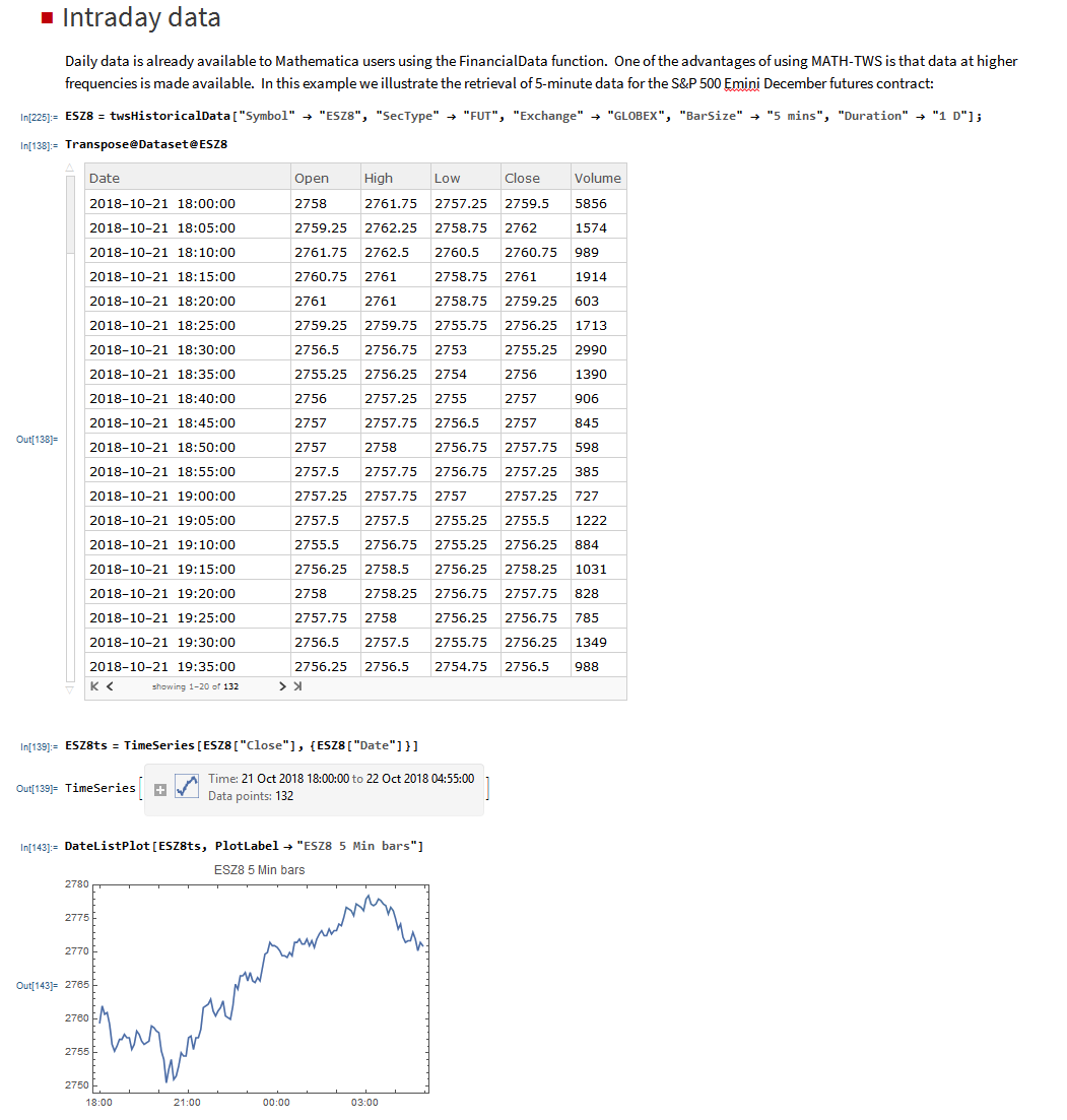
First, let’s look the returns in the ETF portfolios measured using continuous compounding.

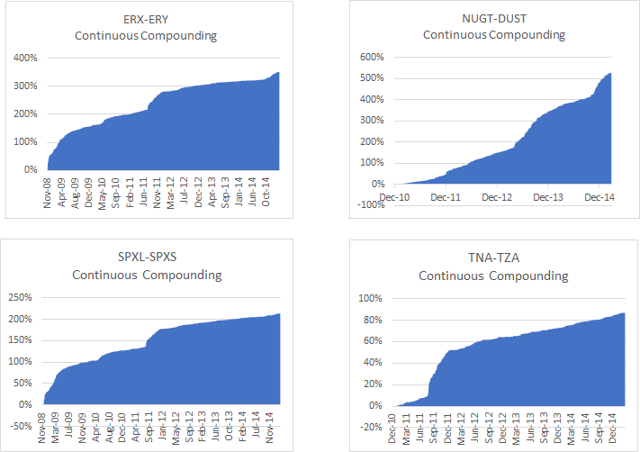
Source: Yahoo! Finance

The portfolio returns look very impressive, with CAGRs ranging from around 20% for the short TNA-TZA pair, to over 124% for the short NUGT-DUST pair. Sharpe ratios, too, appear abnormally large, ranging from 4.5 for the ERX-ERY short pair to 8.4 for NUGT-DUST.

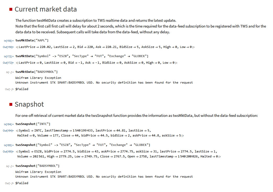
Now let’s look at the performance of the same portfolios measured using daily compounding.

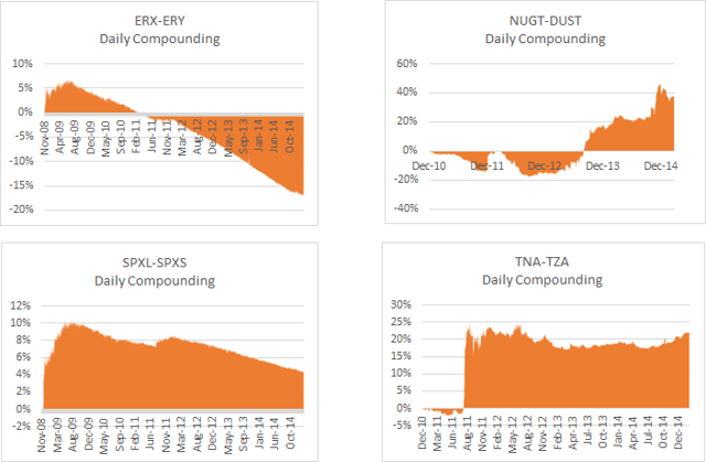
Source: Yahoo! Finance

It’s an altogether different picture. None of the portfolios demonstrate an attract performance record and indeed in two cases the CAGR is negative.

What’s going on?

Stock Loan Costs

Before providing the explanation, let’s just get one important detail out of the way. Since you are shorting both legs of the ETF pairs, you will be faced with paying stock borrow costs. Borrow costs for leveraged ETFs can be substantial and depending on market conditions amount to as much as 10% per annum, or more.

In computing the portfolio returns in both the continuous and daily compounding scenarios I have deducted annual stock borrow costs based on recent average quotes from Interactive Brokers, as follows:

ERX-ERY: 14%
NUGT-DUST: 16%
SXPL-SPXS: 8%
TNA-TZA: 8%

It’s All About Compounding and Rebalancing

The implicit assumption in the computation of the daily compounded returns shown above is that you are rebalancing the portfolios each day. That is to say, it is assumed that at the end of each day you buy or sell sufficient quantities of shares of each ETF to maintain an equal $ value in both legs.

In the case of continuously compounded returns the assumption you are making is that you maintain an equal $ value in both legs of the portfolio at every instant. Clearly that is impossible.

Ok, so if the results from low frequency rebalancing are poor, while the results for instantaneous rebalancing are excellent, it is surely just a question of rebalancing the portfolio as frequently as is practically possible. While we may not be able to achieve the ideal result from continuous rebalancing, the results we can achieve in practice will reflect how close we can come to that ideal, right?

Unfortunately, not.

Because, while we have accounted for stock borrow costs, what we have ignored in the analysis so far are transaction costs.

Transaction Costs

With daily rebalancing transaction costs are unlikely to be a critical factor – one might execute a single trade towards the end of the trading session. But in the continuous case, it’s a different matter altogether.

Let’s use the SPXL-SPXS pair as an illustration. When the S&P 500 index declines, the value of the SPXL ETF will fall, while the value of the SPXS ETF will rise. In order to maintain the same $ value in both legs you will need to sell more shares in SPXL and buy back some shares in SPXS. If the market trades up, SPXL will increase in value, while the price of SPXS will fall, requiring you to buy back some SPXL shares and sell more SPXS.

In other words, to rebalance the portfolio you will always be trying to sell the ETF that has declined in price, while attempting to buy the inverse ETF that has appreciated. It is often very difficult to execute a sale in a declining stock at the offer price, or buy an advancing stock at the inside bid. To be sure of completing the required rebalancing of the portfolio, you are going to have to buy at the ask price and sell at the bid price, paying the bid-offer spread each time.

Spreads in leveraged ETF products tend to be large, often several pennies. The cumulative effect of repeatedly paying the bid-ask spread, while taking trading losses on shares sold at the low or bought at the high, will be sufficient to overwhelm the return you might otherwise hope to make from the ETF decay.

And that’s assuming the best case scenario that shares are always available to short. Often they may not be: so that, if the market trades down and you need to sell more SPXL, there may be none available and you will be unable to rebalance your portfolio, even if you were willing to pay the additional stock loan costs and bid-ask spread.

A Lose-Lose Proposition

So, in summary: if you rebalance infrequently you will avoid excessive transaction costs; but the $ imbalance that accrues over the course of a trading day will introduce a market bias in the portfolio. That can hurt portfolio returns very badly if you get caught on the wrong side of a major market move. The results from daily rebalancing for the illustrative pairs shown above indicate that this is likely to happen all too often.

On the other hand, if you try to maintain market neutrality in the portfolio by rebalancing at high frequency, the returns you earn from decay will be eaten up by transaction costs and trading losses, as you continuously sell low and buy high, paying the bid-ask spread each time.

Either way, you lose.

Ok, what about if you reverse the polarity of the portfolio, going long both legs? Won’t that avoid the very high stock borrow costs and put you in a better position as regards the transaction costs involved in rebalancing?

Yes, it will. Because, you will be selling when the market trades up and buying when it falls, making it much easier to avoid paying the bid-ask spread. You will also tend to make short term trading profits by selling high and buying low. Unfortunately, you may not be surprised to learn, these advantages are outweighed by the cost of the decay incurred in both legs of the long ETF portfolio.

In other words: you can expect to lose if you are short; and lose if you are long!

An Analogy from Option Theory

To anyone with a little knowledge of basic option theory, what I have been describing should sound like familiar territory.

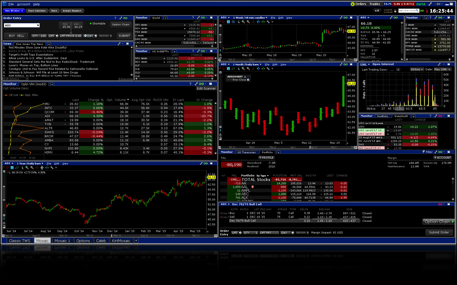
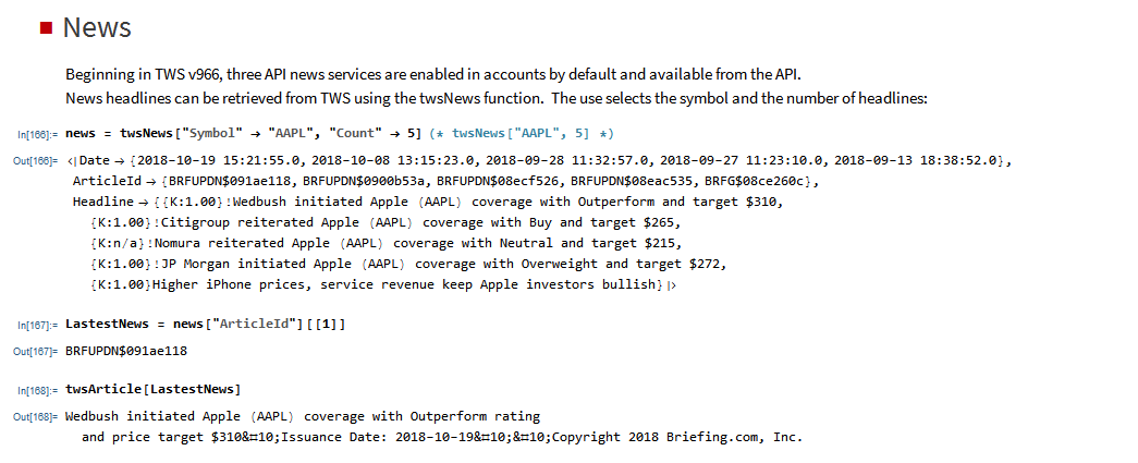
Being short the ETF pair is like being short an option (actually a pair of call and put options, called a straddle). You earn decay, or Theta, for those familiar with the jargon, by earning the premium on the options you have sold; but at the risk of being short Gamma – which measures your exposure to a major market move.

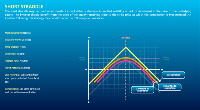
Source: Interactive Brokers

You can hedge out the portfolio’s Gamma exposure by trading the underlying securities – the ETF pair in this case – and when you do that you find yourself always having to sell at the low and buy at the high. If the options are fairly priced, the option decay is enough, but not more, to compensate for the hedging cost involved in continuously trading the underlying.

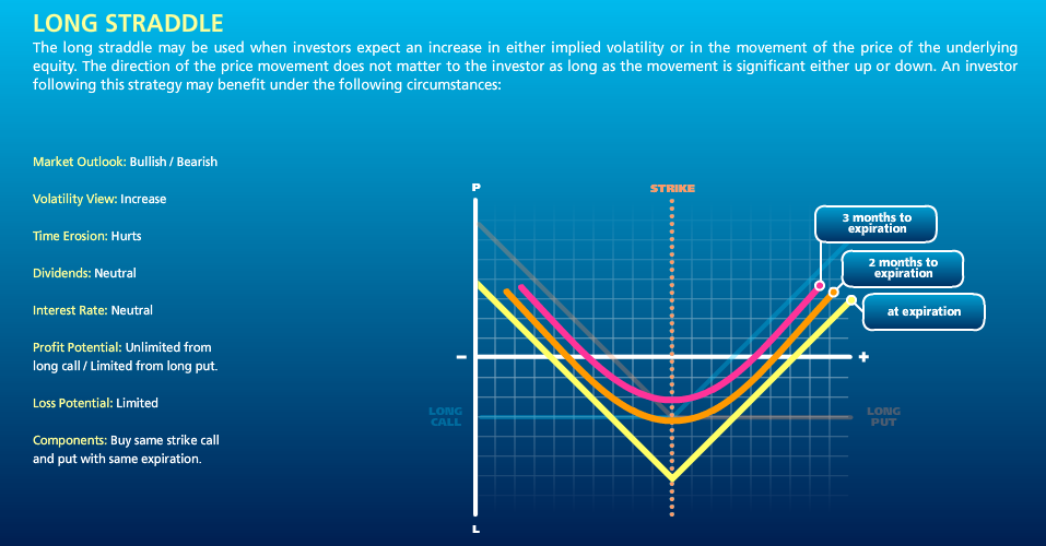
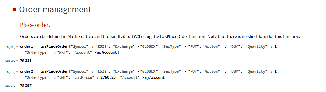
Conversely, being long the ETF pair is like being long a straddle on the underling pair. You now have positive Gamma exposure, so your portfolio will make money from a major market move in either direction. However, the value of the straddle, initially the premium you paid, decays over time at a rate Theta (also known as the “bleed”).

Source: Interactive Brokers

You can offset the bleed by performing what is known as Gamma trading. When the market trades up your portfolio delta becomes positive, i.e. an excess $ value in the long ETF leg, enabling you to rebalance your position by selling excess deltas at the high. Conversely, when the market trades down, your portfolio delta becomes negative and you rebalance by buying the underlying at the current, reduced price. In other words, you sell at the high and buy at the low, typically making money each time. If the straddle is fairly priced, the profits you make from Gamma trading will be sufficient to offset the bleed, but not more.

Typically, the payoff from being short options – being short the ETF pair – will show consistent returns for sustained periods, punctuated by very large losses when the market makes a significant move in either direction.

Conversely, if you are long options – long the ETF pair – you will lose money most of the time due to decay and occasionally make a very large profit.

In an efficient market in which securities are fairly priced, neither long nor short option strategy can be expected to dominate the other in the long run. In fact, transaction costs will tend to produce an adverse outcome in either case! As with most things in life, the house is the player most likely to win.

Developing a Leveraged ETF Strategy that Works

Investors shouldn’t be surprised that it is hard to make money simply by shorting leveraged ETF pairs, just as it is hard to make money by selling options, without risking blowing up your account.

And yet, many traders do trade options and often manage to make substantial profits. In some cases traders are simply selling options, hoping to earn substantial option premiums without taking too great a hit when the market explodes. They may get away with it for many years, before blowing up. Indeed, that has been the case since 2009. But who would want to be an option seller here, with the market at an all-time high? It’s simply far too risky.

The best option traders make money by trading both the long and the short side. Sure, they might lean in one direction or the other, depending on their overall market view and the opportunities they find. But they are always hedged, to some degree. In essence what many option traders seek to do is what is known as relative value trading – selling options they regard as expensive, while hedging with options they see as being underpriced. Put another way, relative value traders try to buy cheap Gamma and sell expensive Theta.

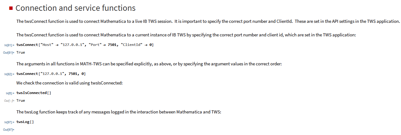
This is how one can thread the needle in leveraged ETF strategies. You can’t hope to make money simply by being long or short all the time – you need to create a long/short ETF portfolio in which the decay in the ETFs you are short is greater than in the ETFs you are long. Such a strategy is, necessarily, tactical: your portfolio holdings and net exposure will likely change from long to short, or vice versa, as market conditions shift. There will be times when you will use leverage to increase your market exposure and occasions when you want to reduce it, even to the point of exiting the market altogether.

If that sounds rather complicated, I’m afraid it is. I have been developing and trading arbitrage strategies of this kind since the early 2000s, often using sophisticated option pricing models. In 2012 I began trading a volatility strategy in ETFs, using a variety of volatility ETF products, in combination with equity and volatility index futures.

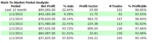
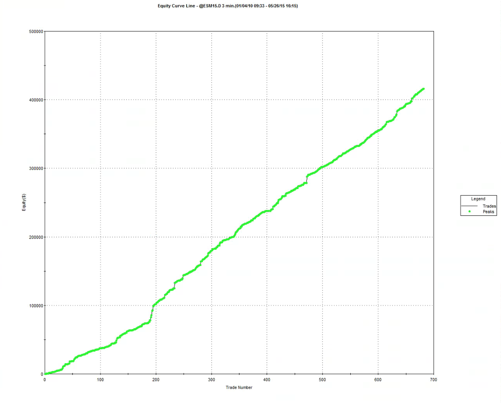
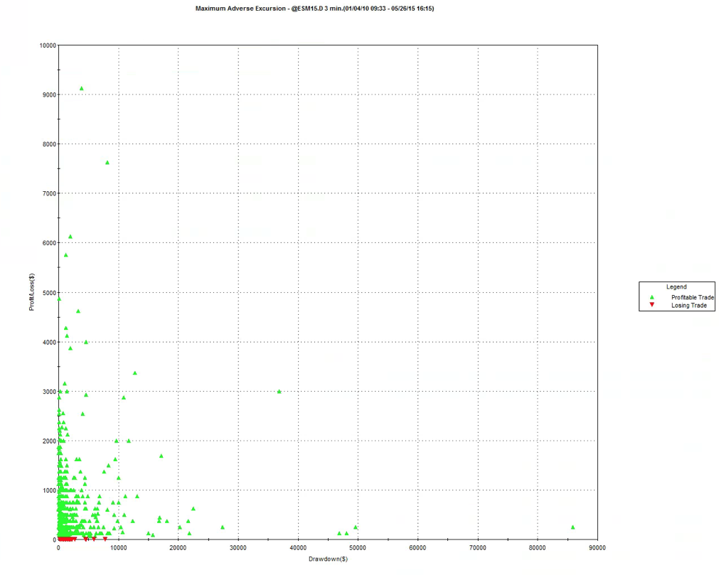
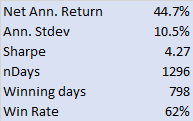
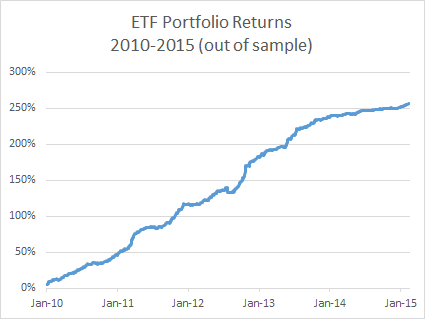
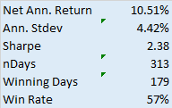
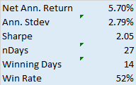
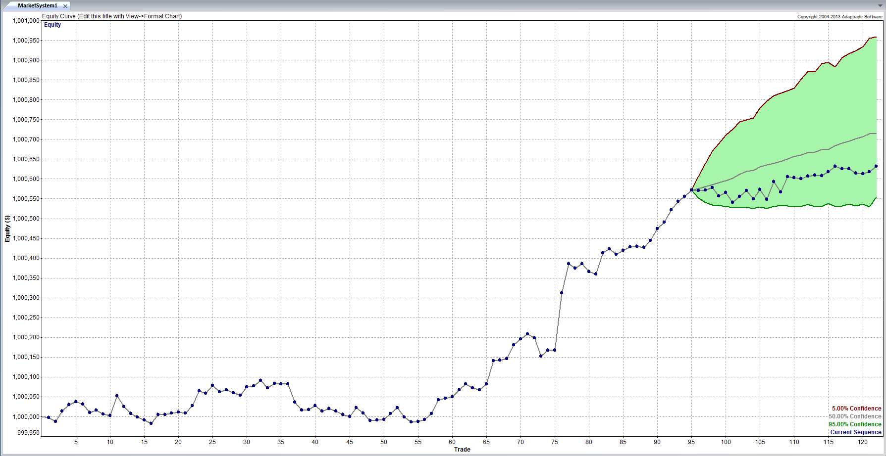
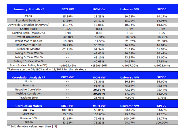
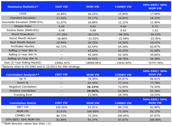
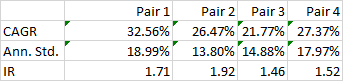
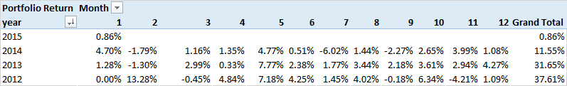
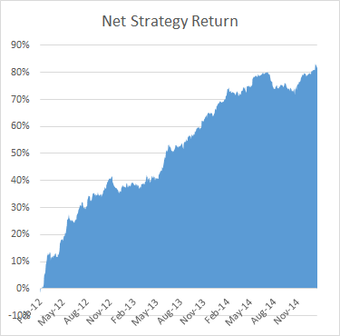
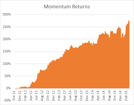
I have reproduced the results from that strategy below, to give some indication of what is achievable in the ETF space using relative value arbitrage techniques.

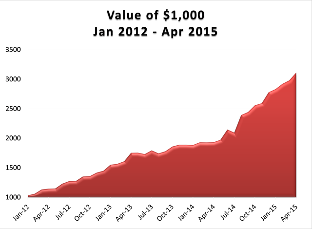Source: Systematic Strategies, LLC

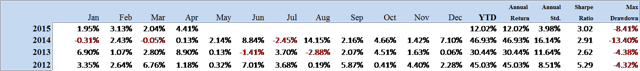
Source: Systematic Strategies LLC

Conclusion

There are no free lunches in the market. The apparent high performance of strategies that engage systematically in shorting leveraged ETFs is an illusion, based on a failure to quantify the full costs of portfolio rebalancing.

The payoff from a short leveraged ETF pair strategy will be comparable to that of a short straddle position, with positive decay (Theta) and negative Gamma (exposure to market moves). Such a strategy will produce positive returns most of the time, punctuated by very large drawdowns.

The short Gamma exposure can be mitigated by continuously rebalancing the portfolio to maintain dollar neutrality. However, this will entail repeatedly buying ETFs as they trade up and selling them as they decline in value. The transaction costs and trading losses involved in continually buying high and selling low will eat up most, if not all, of the value of the decay in the ETF legs.

A better approach to trading ETFs is relative value arbitrage, in which ETFs with high decay rates are sold and hedged by purchases of ETFs with relatively low rates of decay.

An example given of how this approach has been applied successfully in volatility ETFs since 2012.

November 13, 2018

Is Your Trading Strategy Still Working?

The Challenge of Validating Strategy Performance

One of the challenges faced by investment strategists is to assess whether a strategy is continuing to perform as it should. This applies whether it is a new strategy that has been backtested and is now being traded in production, or a strategy that has been live for a while.
All strategies have a limited lifespan. Markets change, and a trading strategy that can’t accommodate that change will get out of sync with the market and start to lose money. Unless you have a way to identify when a strategy is no longer in sync with the market, months of profitable trading can be undone very quickly.

The issue is particularly important for quantitative strategies. Firstly, quantitative strategies are susceptible to the risk of over-fitting. Secondly, unlike a strategy based on fundamental factors, it may be difficult for the analyst to verify that the drivers of strategy profitability remain intact.

Savvy investors are well aware of the risk of quantitative strategies breaking down and are likely to require reassurance that a period of underperformance is a purely temporary phenomenon.

It might be tempting to believe that you will simply stop trading when the strategy stops working. But given the stochastic nature of investment returns, how do you distinguish a losing streak from a system breakdown?

Stochastic Process Control

One approach to the problem derives from the field of Monte Carlo simulation and stochastic process control. Here we random draw samples from the distribution of strategy returns and use these to construct a prediction envelope to forecast the range of future returns. If the equity curve of the strategy over the forecast period falls outside of the envelope, it would raise serious concerns that the strategy may have broken down. In those circumstances you would almost certainly want to trade the strategy in smaller size for a while to see if it recovers, or even exit the strategy altogether it it does not.

I will illustrate the procedure for the long/short ETF strategy that I described in an earlier post, making use of Michael Bryant’s excellent Market System Analyzer software.

To briefly refresh, the strategy is built using cointegration theory to construct long/short portfolios is a selection of ETFs that provide exposure to US and international equity, currency, real estate and fixed income markets. The out of sample back-test performance of the strategy is very encouraging:

There was evidently a significant slowdown during 2014, with a reduction in the risk-adjusted returns and win rate for the strategy:

This period might itself have raised questions about the continuing effectiveness of the strategy. However, we have the benefit of hindsight in seeing that, during the first two months of 2015, performance appeared to be recovering.

Consequently we put the strategy into production testing at the beginning of March 2015 and we now wish to evaluate whether the strategy is continuing on track. The results indicate that strategy performance has been somewhat weaker than we might have hoped, although this is compensated for by a significant reduction in strategy volatility, so that the net risk-adjusted returns remain somewhat in line with recent back-test history.

Using the MSA software we sample the most recent back-test returns for the period to the end of Feb 2015, and create a 95% prediction envelope for the returns since the beginning of March, as follows:

As we surmised, during the production period the strategy has slightly underperformed the projected median of the forecast range, but overall the equity curve still falls within the prediction envelope. As this stage we would tentatively conclude that the strategy is continuing to perform within expected tolerance.

Had we seen a pattern like the one shown in the chart below, our conclusion would have been very different.

As shown in the illustration, the equity curve lies below the lower boundary of the prediction envelope, suggesting that the strategy has failed. In statistical terms, the trades in the validation segment appear not to belong to the same statistical distribution of trades that preceded the validation segment.

This strategy failure can also be explained as follows: The equity curve prior to the validation segment displays relatively little volatility. The drawdowns are modest, and the equity curve follows a fairly straight trajectory. As a result, the prediction envelope is fairly narrow, and the drawdown at the start of the validation segment is so large that the equity curve is unable to rise back above the lower boundary of the envelope. If the history prior to the validation period had been more volatile, it’s possible that the envelope would have been large enough to encompass the equity curve in the validation period.

CONCLUSION

Systematic trading has the advantage of reducing emotion from trading because the trading system tells you when to buy or sell, eliminating the difficult decision of when to “pull the trigger.” However, when a trading system starts to fail a conflict arises between the need to follow the system without question and the need to stop following the system when it’s no longer working.

Stochastic process control provides a technical, objective method to determine when a trading strategy is no longer working and should be modified or taken offline. The prediction envelope method extrapolates the past trade history using Monte Carlo analysis and compares the actual equity curve to the range of probable equity curves based on the extrapolation.

Next we will look at nonparametric distributions tests as an alternative method for assessing strategy performance.

November 6, 2018

The Lazarus Effect

A perennial favorite with investors, presumably because they are easy to understand and implement, are trades based on a regularly occurring pattern, preferably one that is seasonal in nature. A well-known example is the Christmas effect, wherein equities generally make their highest risk-adjusted returns during the month of December (and equity indices make the greater proportion of their annual gains in the period from November to January).

As we approach the Easter holiday I thought I might join in the fun with a trade of my own. There being not much new under the sun, I can assume that there is some ancient trader’s almanac that documents the effect I am about to describe. If so, I apologize in advance if this is duplicative.

The Pattern of Returns in the S&P 500 Index Around Easter

I want to look at the pattern of pre- and post- Easter returns in the S&P 500 index using weekly data from 1950 (readers can of course substitute the index, ETF or other tradable security in a similar analysis).

The first question is whether there are significant differences (economic and statistical) in index returns in the weeks before and after Easter, compared to a regular week.

It is perhaps not immediately apparent from the smooth histogram plot above, but a whisker plot gives a clearer indication of the disparity in the distributions of returns in the post-Easter week vs. regular weeks.

It is evident that chief distinction is not in the means of the distributions, but in their variances.

A t-test (with unequal variances) confirms that the difference in average returns in the index in the post-Easter week vs. normal weeks is not statistically significant.

It appears that there is nothing special about Index returns in the post-Easter period.

The Lazarus Effect

Hold on – not so fast. Suppose we look at conditional returns: that is to say, we consider returns in the post-Easter week for holiday periods in which the index sold off in the week prior to Easter.

There are 26 such periods in the 65 years since 1950 and when we compare the conditional distribution of index returns for these periods against the unconditional distribution of weekly returns we appear to find significant differences in the distributions. Not only is the variance of the conditional returns much tighter, the mean is clearly higher than the unconditional weekly returns.

The comparison is perhaps best summarized in the following table. Here we can see that the average conditional return is more than twice that of the unconditional return in the post-Easter week and almost 4x as large as the average weekly return in the index. The standard deviation in conditional returns for the post-Easter week is less than half that of the unconditional weekly return, producing and information ratio that is almost 10x larger. Furthermore, of the 26 periods in which the index return in the week prior to Easter was negative, 22 (85%) produced a positive return in the week after Easter (compared to a win rate of only 57% for unconditional weekly returns.

A t-test of conditional vs. unconditional weekly returns confirms that the 58bp difference in conditional vs unconditional (all weeks) average returns is statistically significant at the 0.2% level.

Our initial conclusion, therefore, is that there appears to be a statistically significant pattern in the conditional returns in the S&P 500 index around the post-Easter week. Specifically, the returns in the post-Easter week tend to be much higher than average for periods in which the pre-Easter weekly returns were negative.

More simply, the S&P 500 index tends to rebound strongly in the week after Easter – a kind of “Lazarus” effect.

Lazarus – Or Not?

Hold on – not so fast. What’s so special about Easter? Yes, I realize it’s topical. But isn’t this so-called Lazarus effect just a manifestation of the usual mean-reversion in equity index returns? There is a tendency for weekly returns in the S&P 500 index to “correct” in the week after a downturn. Maybe the Lazarus effect isn’t specific to Easter.

To examine this hypothesis we need to compare two sets of conditional weekly returns in the S&P 500 index:

A: Weeks in which the prior week’s return was negative

B: the subset of A which contains only post-Easter weeks

If the difference in average returns for sets A and B is not statistically significant, we would conclude that the so-called Lazarus effect is just a manifestation of the commonplace mean reversion in weekly returns. Only if the average return for the B data set is significant higher than that for set A would we be able to conclude that, in addition to normal mean reversion at weekly frequency, there is an incremental effect specific to the Easter period – the Lazarus effect.

Let’s begin by establishing that there is a statistically significant mean reversion effect in weekly returns in the S&P 500 Index. Generally, we expect a fall in the index to be followed by a rise (and perhaps vice versa). So we need to compare the returns in the index for weeks in which the preceding week’s return was positive, vs weeks in which the preceding week’s return was negative. The t-test below shows the outcome.

The average return in weeks following a downturn is approximately double that during weeks following a rally and the effect is statistically significant at the 3% level.

Given that result, is there any incremental “Lazarus” effect around Easter? We test that hypothesis by comparing the average returns during the 26 post-Easter weeks which were preceded by a downturn in the index against the average return for all 1,444 weeks which followed a decline in the index.

The t-test shown in the table below confirms that conditional returns in post-Easter weeks are approximately 3x larger on average than returns for all weeks that followed a decline in the index.

Lazarus, it appears, is alive and well.

Happy holidays, all.

October 30, 2018

Combining Momentum and Mean Reversion Strategies

The Fama-French World

For many years now the “gold standard” in factor models has been the 1996 Fama-French 3-factor model:
Here r is the portfolio’s expected rate of return, R_f is the risk-free return rate, and K_m is the return of the market portfolio. The “three factor” β is analogous to the classical β but not equal to it, since there are now two additional factors to do some of the work. SMB stands for “Small [market capitalization] Minus Big” and HML for “High [book-to-market ratio] Minus Low”; they measure the historic excess returns of small caps over big caps and of value stocks over growth stocks. These factors are calculated with combinations of portfolios composed by ranked stocks (BtM ranking, Cap ranking) and available historical market data. The Fama–French three-factor model explains over 90% of the diversified portfolios in-sample returns, compared with the average 70% given by the standard CAPM model.

The 3-factor model can also capture the reversal of long-term returns documented by DeBondt and Thaler (1985), who noted that extreme price movements over long formation periods were followed by movements in the opposite direction. (Alpha Architect has several interesting posts on the subject, including this one).

Fama and French say the 3-factor model can account for this. Long-term losers tend to have positive HML slopes and higher future average returns. Conversely, long-term winners tend to be strong stocks that have negative slopes on HML and low future returns. Fama and French argue that DeBondt and Thaler are just loading on the HML factor.

Enter Momentum

While many anomalies disappear under tests, shorter term momentum effects (formation periods ~1 year) appear robust. Carhart (1997) constructs his 4-factor model by using FF 3-factor model plus an additional momentum factor. He shows that his 4-factor model with MOM substantially improves the average pricing errors of the CAPM and the 3-factor model. After his work, the standard factors of asset pricing model are now commonly recognized as Value, Size and Momentum.

Combining Momentum and Mean Reversion

In a recent post, Alpha Architect looks as some possibilities for combining momentum and mean reversion strategies. They examine all firms above the NYSE 40th percentile for market-cap (currently around $1.8 billion) to avoid weird empirical effects associated with micro/small cap stocks. The portfolios are formed at a monthly frequency with the following 2 variables:

Momentum = Total return over the past twelve months (ignoring the last month)
Value = EBIT/(Total Enterprise Value)

They form the simple Value and Momentum portfolios as follows:

EBIT VW = Highest decile of firms ranked on Value (EBIT/TEV). Portfolio is value-weighted.
MOM VW = Highest decile of firms ranked on Momentum. Portfolio is value-weighted.
Universe VW = Value-weight returns to the universe of firms.
SP500 = S&P 500 Total return

The results show that the top decile of Value and Momentum outperformed the index over the past 50 years. The Momentum strategy has stronger returns than value, on average, but much higher volatility and drawdowns. On a risk-adjusted basis they perform similarly. The researchers then form the following four portfolios:

EBIT VW = Highest decile of firms ranked on Value (EBIT/TEV). Portfolio is value-weighted.
MOM VW = Highest decile of firms ranked on Momentum. Portfolio is value-weighted.
COMBO VW = Rank firms independently on both Value and Momentum. Add the two rankings together. Select the highest decile of firms ranked on the combined rankings. Portfolio is value-weighted.
50% EBIT/ 50% MOM VW = Each month, invest 50% in the EBIT VW portfolio, and 50% in the MOM VW portfolio. Portfolio is value-weighted.

With the following results:

The main takeaways are:

The combined ranked portfolio outperforms the index over the same time period.
However, the combination portfolio performs worse than a 50% allocation to Value and a 50% allocation to Momentum.

A More Sophisticated Model

Yangru Wu of Rutgers has been doing interesting work in this area over the last 15 years, or more. His 2005 paper (with Ronald Balvers), Momentum and mean reversion across national equity markets, considers joint momentum and mean-reversion effects and allows for complex interactions between them. Their model is of the form where the excess return for country i (relative to the global equity portfolio) is represented by a combination of mean-reversion and autoregressive (momentum) terms. Balvers and Wu find that combination momentum-contrarian strategies, used to select from among 18 developed equity markets at a monthly frequency, outperform both pure momentum and pure mean-reversion strategies. The results continue to hold after corrections for factor sensitivities and transaction costs. The researchers confirm that momentum and mean reversion occur in the same assets. So in establishing the strength and duration of the momentum and mean reversion effects it becomes important to control for each factor’s effect on the other. The momentum and mean reversion effects exhibit a strong negative correlation of 35%. Accordingly, controlling for momentum accelerates the mean reversion process, and controlling for mean reversion may extend the momentum effect.

Momentum, Mean Reversion and Volatility

The presence of strong momentum and mean reversion in volatility processes provides a rationale for the kind of volatility strategy that we trade at Systematic Strategies. One sophisticated model is the Range Based EGARCH model of Alizadeh, Brandt, and Diebold (2002) . The model posits a two-factor volatility process in which a short term, transient volatility process mean-reverts to a stochastic long term mean process, which may exhibit momentum, or long memory effects (details here).

In our volatility strategy we model mean reversion and momentum effects derived from the level of short and long term volatility-of-volatility, as well as the forward volatility curve. These are applied to volatility ETFs, including levered ETF products, where convexity effects are also important. Mean reversion is a well understood phenomenon in volatility, as, too, is the yield roll in volatility futures (which also impacts ETF products like VXX and XIV).

Momentum effects are perhaps less well researched in this context, but our research shows them to be extremely important. By way of illustration, in the chart below I have isolated the (gross) returns generated by one of the momentum factors in our model.

October 23, 2018October 23, 2018

Developing Long/Short ETF Strategies

Recently I have been working on the problem of how to construct large portfolios of cointegrated securities. My focus has been on ETFs rather that stocks, although in principle the methodology applies equally well to either, of course.

My preference for ETFs is due primarily to the fact that it is easier to achieve a wide diversification in the portfolio with a more limited number of securities: trading just a handful of ETFs one can easily gain exposure, not only to the US equity market, but also international equity markets, currencies, real estate, metals and commodities. Survivorship bias, shorting restrictions and security-specific risk are also less of an issue with ETFs than with stocks (although these problems are not too difficult to handle).

On the downside, with few exceptions ETFs tend to have much shorter histories than equities or commodities. One also has to pay close attention to the issue of liquidity. That said, I managed to assemble a universe of 85 ETF products with histories from 2006 that have sufficient liquidity collectively to easily absorb an investment of several hundreds of millions of dollars, at minimum.

The Cardinality Problem

The basic methodology for constructing a long/short portfolio using cointegration is covered in an earlier post. But problems arise when trying to extend the universe of underlying securities. There are two challenges that need to be overcome.

The first issue is that, other than the simple regression approach, more advanced techniques such as the Johansen test are unable to handle data sets comprising more than about a dozen securities. The second issue is that the number of possible combinations of cointegrated securities quickly becomes unmanageable as the size of the universe grows. In this case, even taking a subset of just six securities from the ETF universe gives rise to a total of over 437 million possible combinations (85! / (79! * 6!). An exhaustive test of all the possible combinations of a larger portfolio of, say, 20 ETFs, would entail examining around 1.4E+19 possibilities.

Given the scale of the computational problem, how to proceed? One approach to addressing the cardinality issue is sparse canonical correlation analysis, as described in Identifying Small Mean Reverting Portfolios, d’Aspremont (2008). The essence of the idea is something like this. Suppose you find that, in a smaller, computable universe consisting of just two securities, a portfolio comprising, say, SPY and QQQ was found to be cointegrated. Then, when extending consideration to portfolios of three securities, instead of examining every possible combination, you might instead restrict your search to only those portfolios which contain SPY and QQQ. Having fixed the first two selections, you are left with only 83 possible combinations of three securities to consider. This process is repeated as you move from portfolios comprising 3 securities to 4, 5, 6, … etc.

Other approaches to the cardinality problem are possible. In their 2014 paper Sparse, mean reverting portfolio selection using simulated annealing, the Hungarian researchers Norbert Fogarasi and Janos Levendovszky consider a new optimization approach based on simulated annealing. I have developed my own, hybrid approach to portfolio construction that makes use of similar analytical methodologies. Does it work?

A Cointegrated Long/Short ETF Basket

Below are summarized the out-of-sample results for a portfolio comprising 21 cointegrated ETFs over the period from 2010 to 2015. The basket has broad exposure (long and short) to US and international equities, real estate, currencies and interest rates, as well as exposure in banking, oil and gas and other specific sectors.

The portfolio was constructed using daily data from 2006 – 2009, and cointegration vectors were re-computed annually using data up to the end of the prior year. I followed my usual practice of using daily data comprising “closing” prices around 12pm, i.e. in the middle of the trading session, in preference to prices at the 4pm market close. Although liquidity at that time is often lower than at the close, volatility also tends to be muted and one has a period of perhaps as much at two hours to try to achieve the arrival price. I find this to be a more reliable assumption that the usual alternative.

The risk-adjusted performance of the strategy is consistently outstanding throughout the out-of-sample period from 2010. After a slowdown in 2014, strategy performance in the first quarter of 2015 has again accelerated to the level achieved in earlier years (i.e. with a Sharpe ratio above 4).

Another useful test procedure is to compare the strategy performance with that of a portfolio constructed using standard mean-variance optimization (using the same ETF universe, of course). The test indicates that a portfolio constructed using the traditional Markowitz approach produces a similar annual return, but with 2.5x the annual volatility (i.e. a Sharpe ratio of only 1.6). What is impressive about this result is that the comparison one is making is between the out-of-sample performance of the strategy vs. the in-sample performance of a portfolio constructed using all of the available data.

Having demonstrated the validity of the methodology, at least to my own satisfaction, the next step is to deploy the strategy and test it in a live environment. This is now under way, using execution algos that are designed to minimize the implementation shortfall (i.e to minimize any difference between the theoretical and live performance of the strategy). So far the implementation appears to be working very well.

Once a track record has been built and audited, the really hard work begins: raising investment capital!

October 22, 2018October 22, 2018

MATH-TWS: Connecting Wolfram Mathematica to IB TWS

Mathematica can now connect to Interactive Brokers Trader Workstation

At long last, it’s here!

MATH-TWS is a new Mathematica package that connects Wolfram Mathematica to the Interactive Brokers TWS platform via the C++ API. It enables the user to retrieve information from TWS on accounts, portfolios and positions, as well as historical and real-time market data. MATH-TWS also enables the user to place and amend orders and obtain execution confirmations from Mathematica.

In the following sections we will illustrate the functionality of the MATH-TWS package using the full functional form and show the abbreviated equivalent form in comments.

Conclusions: Connecting Mathematica to IB TWS

I have wanted a way to connect Wolfram Mathematica to Interactive Brokers’ Trader Workstation for the longest time. Now that it is finally available with MATH-TWS I am excited by the possibilities for Mathematica users.

The first release of MATH-TWS will be available within a couple of weeks. Anyone interested in licensing a copy should email algorithmicexecution@gmail.com with MATH-TWS in the subject line.

October 16, 2018

Algorithmic Trading

MOVING FROM RESEARCH TO TRADING

I have written recently about the comparative advantages of different programming languages in the context of research and trading (see here). My sense of it is that there is no single “ideal” programming language – the best strategy is to pick an appropriate tool for the job and there are usually several reasonable choices one could make.

If you are engaged in econometrics research, you might choose a package like RATS, Eviews, Gauss, or Prof. James Davidson’s excellent and inexpensive TSM, which I have used for many years and can recommend highly. For a latency-sensitive high frequency trading application, you will probably want to use something like C++, or possibly a 3rd party algo system like Apama or Tethys. But for algorithmic trading systems of intermediate frequency the choice appears almost unlimited.

The problem with retail trading tools like TradeStation, Multicharts, or Amibroker, is that they are designed primarily for single-asset strategies. That may be ok for futures trading,where more often than not the focus is on a single underlying, but in equities the opposite is true. Using one of these products to develop and implement a pairs trading strategy is a stretch. As for portfolio analytics – forget it.

This is where more general, high level languages like R, Matlab or Mathematica come in: their greater power and flexibility is handling large, multivariate data sets makes it much more straightforward to develop portfolio strategies. And they can often bridge the gap between R&D and implementation quite easily: code that was used in the research stage can often be quickly re-tooled to work in a production version of the system. As for production systems, there is now a significant cottage industry of traders who use Matlab in algo trading. R has a similar following (see here).

In addition to parallelizing the code (for use with the Parallel Computing Toolbox) to speed up the research phase, you might also want to implement a hybrid system by re-coding the slower routines in C++, to create a mex file (for details see here). Matlab’s Profiler is a useful tool for identifying code bottlenecks. In a recent piece of research in which I was evaluating over 30,000,000 cointegrated portfolios, I discovered to my surprise that the main code bottleneck was the multiple calls to Matlab’s std function, a problem easily fixed with a few lines of C++ code. The resulting hybrid program executed at more than twice the speed – important when your run time might be several hours, or even days.

HOOKING UP THE EXECUTION PLATFORM

The main challenge for developers using generic tools like Mathematica, Matlab or R is the implementation stage of the project. Providing connectivity to brokerage/execution platforms never seemed high on the list of priorities for Wolfram or Mathworks and things are similarly hit or miss with R.

Belatedly, Mathematica now offers a link to Bloomberg via its Finance Platform. Matlab, meanwhile, offers a Trading Toolbox, which supposedly offers connectivity , not only to Bloomberg, but also Interactive Brokers and Trading Technologies, amongst other platforms. Unfortunately, the toolbox interface to IB appears to rely on outdated 1990s ActiveX technology, which is flakey at best. In tests, I was unable to make progress past the ‘not connected’ error message.

At that point I turned to Yair Altman’s IB-Matlab product. Happily, this uses IB’s Java api, which is a great deal more robust than the ActiveX platform. It’s been some time since I last used IB-Matlab and was pleased to see that Yair has been very busy over the intervening period, building the capabilities of the system and providing very comprehensive documentation for it. With Yair’s help, it took me no time at all to get up and running and within a day or two the system was executing orders flawlessly in IB’s TWS. The relatively few snags I ran into were almost all due to IB’s extremely terse error messaging, which often gives almost no clue as to what the issue might be. Fortunately, Yair is very generous with his time in providing support to his users and his responses to me questions were fast and detailed.

EXECUTION ALGOS

With intermediate systems trading at frequencies of, say, 5-minutes to daily, one has a choice to make as regards execution. Given that the strategy is not very latency sensitive, it is certainly conceivable to develop one’s own execution algos in Matlab. However, platforms like TWS are equipped with native algos, not only from IB, but also other providers like Credit Suisse and Jeffries.

Actually, I have found several of IB’s own algos such as Scaletrader and Accumulate/Distribute to be very effective. Certainly IB seems very proud of them – IB CEO Thomas Peterffy has patented at least one of them. Accumulate/Distribute, for instance, is quite sophisticated, allowing the user to randomize and slice the size and interval between individual orders, use passive or aggressive order types, and pause execution on a news alert, or when the price falls below a moving average, or outside a specified range.

There is much to be said for using algos native to the execution platform rather than reinventing the wheel, providing the cost is reasonable. So, while it is perfectly feasible to build execution algos in Matlab, it typically isn’t necessary – in most cases standard algos will suffice.

There are exceptions, of course. IB doesn’t offer the kind of basket-trading capabilities that are available in advanced algo platforms like Tethys or RediPlus. In those systems, for example, you can set the level of long/short imbalance in the portfolio that you are willing to tolerate and the algo will speed up or slow down execution of trades in individual components of the basket to maintain the dollar imbalance within that tolerance. You can also manage the sector risk dynamically during execution.

Those kind of advanced capabilities don’t come cheap and you wont find them at IB, or any other retail platform. If you need that kind of functionality, for example, because you are trading a long/short equity portfolio within a universe of 200-300 names, your best option is probably to switch to a different execution platform. Otherwise you will need to code a custom algo in your language of choice.

For many quantitative strategies, (at least the low frequency ones) IB’s standard algos are often good enough. The Accumulate/Distribute algo, for instance, will show a visual representation of the progress of the execution of individuals legs of a pairs trade, and it is easy enough to identify a potential imbalance and adjust the algo parameters in real time. If you are only trading pairs, or small portfolios of cointegrated securities, it probably isn’t worthwhile to develop the sophisticated logic that would be required to handle the adjustment of the execution of individual legs of a trade in a fully automated way. A large portfolio would be a different matter, however.

MATLAB EXAMPLE

I thought it might be instructive to take a look at how you might implement the execution of a strategy in Matlab, using IB algos. In the Matlab code fragment below, the (2 x nTickers) array tradeActions contains, in the first row, the action we wish to take (1 = BUY, -1 = SELL, -2 = SELL SHORT) and in the second row the (absolute value of) the number of shares we wish to trade for tickers i =1:nTickers. We break each order up into hundred lots and odd lots, routing the former via IB’s Accumulate/Distribute algo and the latter as passive REL orders (note that A/D will typically randomize the timing of each sub-order, while REL orders are posted directly into the market). The Matlab function AccumulateDistribute implements the most important features of IB’s A/D algo, including random size and time slicing of the order. Orders are submitted as passive REL orders with zero offset (so they will sit on the current bid or ask) – obviously you would typically want to consider allowing some non-zero offset for less liquid securities. It is not hard to envisage how one might further enhance the algo to monitor the progress of the execution and speed up or slow down certain orders accordingly.

A couple of IB api “gotchas” to be aware of:

(i) IB requires unique and monotonically increasing orderIds for each order. One way to do this, suggested by Yair, is to use orderId = round((now-735000)*3e5); This fails when you are submitting a number of orders sequentially at high speed (say in a for loop), where the time increments are sub-second, so you need to pass the orderID back and force a minimal increment, as I have in the code below.

(ii) It is very important to specify the primary exchange of each security: securities with identical tickers can be found trading on different exchanges. Failing to specify the primary exchange in such a case will result in IB rejecting the order with a typically cryptic api message.

Continue reading “Algorithmic Trading”

October 10, 2018October 11, 2018

Cointegration Breakdown

The Low Power of Cointegration Tests

One of the perennial difficulties in developing statistical arbitrage strategies is the lack of reliable methods of estimating a stationary portfolio comprising two or more securities. In a prior post (below) I discussed at some length one of the primary reasons for this, i.e. the lower power of cointegration tests. In this post I want to explore the issue in more depth, looking at the standard Johansen test Procedure to estimate cointegrating vectors.

Johansen Test for Cointegration

Start with some weekly data for an ETF triplet analyzed in Ernie Chan’s book:

After downloading the weekly close prices for the three ETFs we divide the data into 14 years of in-sample data and 1 year out of sample:

We next apply the Johansen test, using code kindly provided by Amanda Gerrish:

We find evidence of up to three cointegrating vectors at the 95% confidence level:

Let’s take a look at the vector coefficients (laid out in rows, in Amanda’s function):

In-Sample vs. Out-of-Sample testing

We now calculate the in-sample and out-of-sample portfolio values using the first cointegrating vector:

The portfolio does indeed appear to be stationary, in-sample, and this is confirmed by the unit root test, which rejects the null hypothesis of a unit root:

Unfortunately (and this is typically the case) the same is not true for the out of sample period:

More Data Doesn’t Help

The problem with the nonstationarity of the out-of-sample estimated portfolio values is not mitigated by adding more in-sample data points and re-estimating the cointegrating vector(s):

We continue to add more in-sample data points, reducing the size of the out-of-sample dataset correspondingly. But none of the tests for any of the out-of-sample datasets is able to reject the null hypothesis of a unit root in the portfolio price process:

The Challenge of Cointegration Testing in Real Time

In our toy problem we know the out-of-sample prices of the constituent ETFs, and can therefore test the stationarity of the portfolio process out of sample. In a real world application, that discovery could only be made in real time, when the unknown, future ETFs prices are formed. In that scenario, all the researcher has to go on are the results of in-sample cointegration analysis, which demonstrate that the first cointegrating vector consistently yields a portfolio price process that is very likely stationary in sample (with high probability).

The researcher might understandably be persuaded, wrongly, that the same is likely to hold true in future. Only when the assumed cointegration relationship falls apart in real time will the researcher then discover that it’s not true, incurring significant losses in the process, assuming the research has been translated into some kind of trading strategy.

A great many analysts have been down exactly this path, learning this important lesson the hard way. Nor do additional “safety checks” such as, for example, also requiring high levels of correlation between the constituent processes add much value. They might offer the researcher comfort that a “belt and braces” approach is more likely to succeed, but in my experience it is not the case: the problem of non-stationarity in the out of sample price process persists.

Conclusion: Why Cointegration Breaks Down

We have seen how a portfolio of ETFs consistently estimated to be cointegrated in-sample, turns out to be non-stationary when tested out-of-sample. This goes to the issue of the low power of cointegration test, and their inability to estimate cointegrating vectors with sufficient accuracy. Analysts relying on standard tests such as the Johansen procedure to design their statistical arbitrage strategies are likely to be disappointed by the regularity with which their strategies break down in live trading.

October 9, 2018

Successful Statistical Arbitrage

I tend not to get involved in Q&A with readers of my blog, or with investors. I am at a point in my life where I spend my time mostly doing what I want to do, rather than what other people would like me to do. And since I enjoy doing research and trading, I try to maximize the amount of time I spend on those activities.

As a business strategy, I wouldn’t necessarily recommend this approach. It’s just something I evolved while learning to play chess: since I had no-one to teach me, I had to learn everything for myself and this involved studying for many, many hours alone.

By contrast, several of the best money managers are also excellent communicators – take Roy Niederhoffer, or Ernie Chan, for example. Having regular, informed communication with your investors is, as smarter managers have realized, a means of building trust and investor loyalty – important factors that come into play during periods when your strategy is underperforming. Not only that, but since communication is two-way, an analyst/manager can learn much from his exchanges with his clients. Knowing how others perceive you – and your competitors – for example, is very useful information. So, too, is information about your competitors’ research ideas, investment strategies and fund performance, which can often be gleaned from discussions with investors. There are plenty of reasons to prefer a policy of regular, open communication.

As a case in point, I was surprised to learn from comments on another research blog that readers drew the conclusion from my previous posts that pursuing the cointegration or Kalman Filter approach to statistical arbitrage was a waste of time. Apparently, my remark to the effect that researchers often failed to pay attention to the net PnL per share in evaluating stat. arb. trading strategies was taken by some to mean that any apparent profitability would always be subsumed within the bid-offer spread. That was not my intention. What I intended to convey was that in some instances, this would be the case – some, but not all.

To illustrate the point, below are the out-of-sample results from a research study applying the Kalman Filter approach for four equity pairs using 5-minute data. For competitive reasons I am unable to identify the specific stocks in each pair, which result from an exhaustive analysis of over 30,000 pairs, but I can say that they are liquid large-cap equities traded in large volume on the US exchanges. The performance numbers are net of transaction costs and are based on the assumption of a 5-minute delay in execution: meaning, a trading signal received at time t is assumed to be executed at time t+5 minutes. This allows sufficient time to leg into each trade passively, in most cases avoiding the bid-offer spread. The net PnL per share is above 1.5c per share for each pair.

While the performance of none of the pairs is spectacular, a combined portfolio has quite attractive characteristics, which include 81% winning months since Jan 2012, a CAGR of over 27% and Information Ratio of 2.29, measured on monthly returns (2.74 based on daily returns).

Finally, I am currently implementing trading of a number of stock portfolios based on static cointegration relationships that have out-of-sample information ratios of between 3 and 4, using daily data.