Month: May 2026

A self-contained synthetic benchmark of a small mask-conditional CNN against calendar-projected linear interpolation and a per-slice SVI fit.

A volatility surface marker is rarely a clean rectangle of quotes. Strikes go unobserved during illiquid hours, wings get crossed and then erased, broker stripes drop out across an entire maturity, and weeklies arrive at the desk with random missingness on top of base quote noise. Anyone calibrating an SVI surface or running an SSVI fit operationally is doing it on top of an upstream repair step, whether that step is explicit or not. The repair step is usually some flavour of local interpolation, sometimes followed by a no-arbitrage projection, sometimes pre-empted by a model-based smoother.

The question I want to put a number on is whether a small learned model can compete with the local approach in this repair role. The reason to ask is that a learned model, in principle, knows something about the joint structure of plausible volatility surfaces that a local interpolator does not — vol surfaces are not arbitrary functions on a (k, T) grid, they have term-structure shape, characteristic skew patterns, ATM smoothness — and a model that has seen a thousand surfaces should be able to use that prior to improve on local interpolation, especially where local data is thin.

The reason to be sceptical is that local methods are very strong at what they do. Linear interpolation in (T, k) is unbiased, has no parameters to overfit, costs nothing operationally, and is hard to beat on smooth surfaces with reasonable observation density. Per-slice SVI gets you smile shape correctly even when only a handful of strikes are observed, provided the slice has enough quotes to fit. Beating both of those baselines requires that the learned prior contributes something local methods cannot — and the most plausible places for that to happen are when local data is too sparse for SVI to fit and too irregular for interpolation to fill the gap cleanly.

This note runs that experiment on synthetic data. It is deliberately a small CNN rather than a U-Net or a VAE, partly because that is the smallest interesting architecture for this problem, and partly because if a small model cannot establish a foothold here, the question of whether to build something larger has a clearer answer than if it can.

The full code is in vol_surface_repair.py; it runs on CPU in roughly four minutes.

Setup

Grid. Maturities and log-moneyness on a 13 × 17 grid: T \in [0.08, 2.0] (years), k \in [-0.45, 0.45]. All surfaces are stored as total variance w(k, T) = \sigma^2(k, T)\, T; evaluation metrics are computed in implied-vol units (\sigma) for interpretability.

Training surfaces. 1600 SSVI surfaces drawn from a fairly tight parameter range:

theta0 = U(0.010, 0.032)        # ATM total variance at front
theta_slope = U(0.020, 0.070)   # linear term in maturity
theta_curve = U(-0.006, 0.010)  # quadratic term
rho = U(-0.72, -0.18)           # skew
eta = U(0.55, 1.55)             # SSVI eta
gamma = U(0.18, 0.62)           # SSVI gamma

Calendar monotonicity is enforced on the clean target via cumulative maximum along T so the model is never rewarded for learning calendar arbitrage from the simulator. A 200-surface validation set, drawn from the same parameter range with different seeds, is held out for best-checkpoint selection.

Test surfaces. Two test families, each with 200 surfaces per cell and seeds independent of training:

• Shifted SSVI — same generator with widened parameter ranges and an occasional maturity-localised bump. The generator is in-distribution in form but stress-tests the boundaries.
• SABR-style event — a separate generator deliberately not identical to SSVI, with square-root maturity decay in ATM vol, stochastic skew term-structure, asymmetric wings, and occasional event-maturity bumps and kinks. This is the out-of-distribution test: smile structure that the model has never seen.

Both families are then perturbed by realistic quote noise (~18 bps in vol space, with wing- and front-end inflation) and masked according to one of two missingness regimes:

• Regular — about 50% observation density, modest wing deletions, occasional broker-style stripes.
• Adversarial — about 18% observation density, large contiguous wing or maturity holes, with a thin ATM spine and a few scattered anchors restored so the problem remains solvable but is genuinely sparse.

The result is a 2 × 2 evaluation: {shifted SSVI, SABR-event} × {regular, adversarial}. The motivation is to disentangle two different ways the repair task can be hard: hard because the model has not seen this surface family before, and hard because the available data is too sparse for any local method to cope.

Baselines. Two of them.

• Calendar-projected linear interpolation: triangulated linear interpolation in (T, k) on observed total variance, with a nearest-neighbour fallback for points outside the convex hull, followed by a cumulative-maximum projection along T to enforce calendar monotonicity. Unparameterised, fast, hard to beat on smooth surfaces.
• Per-slice SVI fit: at each maturity, a coarse raw-SVI grid search over (\rho, m, \sigma) with the best (a, b) solved in closed form by least squares. Faster than nonlinear least squares, adequate as a baseline. Followed by the same calendar projection as interpolation. This is the published-textbook approach to surface repair when you have enough quotes per slice.

Both baselines are evaluated on the same noisy/masked inputs as the CNN.

Model

The repair network is a four-layer 32-channel convolutional network with two output heads — a softplus mean head and a clipped log-variance head:

class RepairCNN(nn.Module):
    def __init__(self, in_channels=4, width=32):
        super().__init__()
        self.backbone = nn.Sequential(
            nn.Conv2d(in_channels, width, 3, padding=1), nn.SiLU(),
            nn.Conv2d(width, width, 3, padding=1), nn.SiLU(),
            nn.Conv2d(width, width, 3, padding=1), nn.SiLU(),
            nn.Conv2d(width, width, 3, padding=1), nn.SiLU(),
        )
        self.mean_head = nn.Conv2d(width, 1, 1)
        self.logvar_head = nn.Conv2d(width, 1, 1)
​
    def forward(self, x):
        z = self.backbone(x)
        mean = F.softplus(self.mean_head(z)) + 1e-5  # w / W_SCALE
        log_var = torch.clamp(self.logvar_head(z), -8.0, 1.5)
        return mean, log_var

The four input channels are the masked observed total variance (normalised by W_SCALE = 0.08), the binary observation mask, and two normalised coordinate channels for maturity and log-moneyness. The mean head outputs normalised total variance; the log-variance head produces a heteroscedastic uncertainty estimate.

The output space is total variance rather than implied vol. Both choices are defensible — a controlled experiment with the same training pipeline run in vol space gives essentially identical missing-point RMSE — and total variance has the practical advantage that calendar-arbitrage and butterfly-arbitrage diagnostics are natural in this space.

The loss is a weighted reconstruction term in the normalised w-space, plus a heteroscedastic Gaussian NLL (turned on after a 10-epoch warmup), plus a calendar-arbitrage penalty (penalising negative differences along T in real-w space), plus a small smoothness regulariser:

def repair_loss(mean_norm, log_var, target_norm, mask, cfg, use_nll):
    weights = 1.0 + (cfg.missing_weight - 1.0) * (1.0 - mask)
    sq = (mean_norm - target_norm)**2
    mse = torch.mean(weights * sq)
    loss = mse
    if use_nll and cfg.nll_weight:
        inv_var = torch.exp(-log_var)
        nll = 0.5 * torch.mean(weights * (sq * inv_var + log_var))
        loss = loss + cfg.nll_weight * nll
    if cfg.calendar_weight:
        loss = loss + cfg.calendar_weight * calendar_penalty_w(mean_norm)
    if cfg.smoothness_weight:
        loss = loss + cfg.smoothness_weight * smoothness_penalty(mean_norm)
    return loss

The missing-cell weight is 5x the observed-cell weight, so the model is explicitly graded on its repair quality rather than its ability to denoise observed quotes. The calendar weight is set to 80, which is high enough to drive raw calendar-violation rates into single digits at evaluation time but not so high that it dominates the reconstruction loss during training. The smoothness term is small (0.05 weight) and exists mainly to discourage high-frequency artefacts at the wings.

Training runs for 60 epochs in a single process with AdamW (lr 1e-3, wd 1e-4) and a cosine annealing schedule. The first 10 epochs run pure MSE; the NLL term turns on afterwards to give the variance head an MSE-stabilised mean to train against. A 200-surface validation set is used for best-checkpoint selection by missing-point RMSE in vol units. Batch size 128, gradient clipping at norm 1.0.

I will say a word about training duration because the result is more sensitive to it than I would like. With only 8 training epochs, the model’s missing-point RMSE on shifted SSVI / regular missing is 0.049 in vol units; at 60 epochs it is 0.018. The convergence is slow and the validation curve is still improving slightly at epoch 60. Sixty epochs is therefore a deliberate choice rather than a generous one — at that point the validation curve has flattened enough that further training mostly trades off in-distribution refinement against out-of-distribution generalisation, with no clear winner.

The 2 × 2 result

Headline numbers: missing-point RMSE in implied-vol units, mean ± standard error across 200 test surfaces per cell. Bold marks the best estimator per row, with ties (within one SE) bolded together.

Four cells, four different stories.

Shifted SSVI / regular. Calendar-projected linear interpolation wins outright: 0.013 versus the CNN’s 0.018. The surfaces here are smooth, the parameter shifts from the training distribution are modest, and roughly half the grid is observed. There is little for a learned prior to add: the local data is dense enough that triangulated interpolation captures essentially all the recoverable structure. The CNN is 40% worse, well outside one SE.

Shifted SSVI / adversarial. The CNN and interpolation are statistically tied (0.053 vs 0.051, within one SE of each other). With observation density at 18% and large contiguous holes, neither method has a clean run, but the CNN’s learned prior on smile shape brings it back into the same neighbourhood as interpolation. The SVI fit is also competitive here, although noisier across surfaces because individual maturity slices sometimes have too few quotes to fit reliably.

SABR-event / regular. SVI wins narrowly (0.019 vs interpolation’s 0.025), the CNN comes in third at 0.067. This is the cell that distinguishes baselines: SVI fits the local smile structure correctly slice-by-slice and pays no penalty for the SABR family being out-of-distribution because it is a per-slice model with no cross-slice prior to mislead it. The CNN, trained only on SSVI surfaces, has learned a prior that does not transfer cleanly to the asymmetric-wings, event-kink SABR family. It is 2.5× worse than SVI here.

SABR-event / adversarial. Interpolation wins (0.068 vs the CNN’s 0.096), with SVI in the middle at 0.078 and noisy because slice-level data is too sparse to fit consistently. The dominant error source for the CNN here is generalisation, not data scarcity. Even with adversarial missingness — exactly the case where one might hope a learned prior contributes most — the OOD penalty dominates.

The pattern across cells is consistent. The CNN is competitive only where its learned prior matches the test distribution and local methods are operating at their weakest. It loses materially when either of those conditions fails. Calendar-projected linear interpolation is the most consistent baseline of the three: it is the best estimator in two cells, statistically tied for best in a third, and the second-best in the fourth.

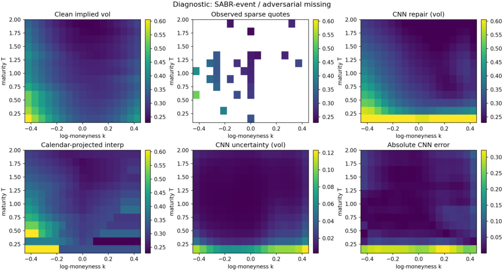
The diagnostic figure below shows a single SABR-event adversarial-missingness example. The observed input has lost a substantial chunk of the wings, the entire long-maturity tail, and the front-maturity strip; what remains is a thin ATM spine and a handful of scattered anchors. The CNN repair is smooth and plausible, with errors concentrated at the front-maturity wings — exactly where the input is most aggressively masked. The uncertainty head correctly flags that region as high-uncertainty. Calendar-projected interpolation produces the characteristic “shelf” artefact at the maturities where the cumulative-max projection has had to adjust the raw output.

Diagnostics

A repair model that minimises missing-point RMSE while producing arbitrageable surfaces and miscalibrated uncertainty is not a usable estimator. The diagnostics below are not the headline; they are the things you have to report in order for the headline to load-bear.

The honest summary, line by line:

Calendar arbitrage. The raw CNN output violates calendar monotonicity in 2–11% of (k, T) edges across the four cells. The cumulative-maximum projection drives this to zero everywhere. The calendar-projection step is therefore doing real work, and the model should not be deployed without it. The training-time calendar penalty is doing partial work — without it, raw violation rates would be substantially higher — but it is not on its own sufficient to produce calendar-monotone output reliably.

Butterfly arbitrage. Even after calendar projection, 5–11% of grid points exhibit g(k) < 0 under the discrete Gatheral–Roper diagnostic, with the worst rates on the SABR cells where the CNN is least confident. The smoothness penalty in the loss does not buy enough convexity to fix this. A real butterfly-arbitrage projection — one that actually projects onto the no-arbitrage manifold along k rather than just regularising — would be the right next step. I have not done it here, and the post-projection g(k)<0 rate is the most concerning single number in this set of diagnostics.

Uncertainty calibration. The heteroscedastic head undercovers. Nominal 80% intervals deliver 28–69% empirical coverage; nominal 95% intervals deliver 41–85%. The error-versus-predicted-sd correlation is positive everywhere (0.64–0.86), so the model is at least directionally aware of where its output is unreliable, but it is overconfident about how unreliable it is — particularly on the OOD SABR cells, where the variance head has nothing to recalibrate against. This is the standard limit of in-training Gaussian NLL: under distribution shift, the variance head is as miscalibrated as the mean head, in the same direction. A held-out conformal step is the obvious fix and would be the cheapest single change to make the uncertainty channel operationally useful.

Stale-quote AUC. A synthetic test: inject stale errors into 8% of observed quotes, run the model on the stale-injected surface, and compute the AUC of the residual |obs – \mu| as a stale-quote score. Numbers come in at 0.55–0.66. Better than chance, but weak — particularly on the OOD SABR cells where the AUC sits just above 0.55. This says the model’s residual is not, on its own, a strong stale-quote detector. A more useful operational stale-detection pipeline would combine the model residual with quote-time and quote-source signals, and the model is contributing a useful but limited fraction of the discriminative signal.

Downstream SVI projection

Surface repair is a means to an end. What the calibration desk usually wants is a smooth, arbitrage-projected SVI surface, not the raw repair output. A repair that is more accurate in the missing-point RMSE sense but less amenable to clean SVI projection might be a worse operational deliverable than the reverse. The right question is not just “how accurate is the repair” but “how good is the SVI fit to the repaired full surface”.

To get at this, I run a per-slice SVI projection on the full repaired surface (CNN or calendar-projected interpolation), then re-score the SVI fit against the held-out missing cells:

The downstream metric does not change the qualitative ranking: CNN-then-SVI narrowly beats interp-then-SVI on the cell where the headline RMSE was already tied (SSVI / adversarial), and loses everywhere else. The CNN is not producing surfaces that are pathologically uncooperative under SVI projection — the SVI residuals follow the missing-point RMSE residuals reasonably faithfully. That is mildly reassuring from a deployment perspective: the choice between estimators is not being secretly arbitraged away by the projection step.

What this experiment shows and does not show

A small mask-conditional CNN, trained on 1600 synthetic SSVI surfaces under explicit calendar and smoothness penalties, with 200 validation surfaces for checkpoint selection, can repair sparse and noisy total-variance surfaces under a tight enough discipline that it:

• produces calendar-monotone output after a cumulative-maximum post-projection (which both baselines also need);
• matches calendar-projected linear interpolation, within statistical noise, on adversarial in-distribution missingness;
• loses to interpolation by roughly 40% on benign in-distribution missingness, where the local-data density is high enough that triangulated interpolation captures essentially all the recoverable structure;
• loses by a factor of 1.4–2.7× on out-of-distribution SABR-style smiles, depending on observation density;
• carries a heteroscedastic uncertainty estimate whose direction is right (positive correlation with error) but whose magnitude is undercalibrated, particularly under distribution shift.

What this experiment does not show, and what I want to be plain about:

It does not show that this kind of CNN-based repair is useful on real data. The synthetic surfaces have no calibration drift, no quote-time-of-day noise, no microstructure asymmetries, no realistic smile dynamics, no hard-to-fit weeklies or single-name idiosyncrasies. The repair task here is pristine compared to anything one would do on production market data. Whether the small relative gap between CNN and interpolation on the adversarial cell survives a real-data test is an open question that this experiment cannot answer.

It does not show that a CNN is the right architecture for this task. A four-layer 32-channel CNN on a 13 × 17 grid is the smallest interesting model for this problem; a U-Net, an attention-conditioned masked decoder, or a conditional VAE all have published precedents in the volatility-repair literature and would be plausible candidates for materially better performance. The choice here was deliberate — keep the model small and the comparison clean — but it is not the architecture I would deploy if I were trying to win the headline number.

It does not show that the SABR-event family is the right test for OOD generalisation. The CNN is being asked to handle smiles whose convexity term-structure and wing asymmetry have a different functional form from anything in its training set. That is a hard test by design, and the gap to SVI on SABR / regular says that what the CNN has learned is closer to “the SSVI smile family” than “smile structure in general”. A more useful experiment would mix multiple smile families during training and re-test on a held-out one.

It does not, on its own, justify a production system. Before this estimator went anywhere near a market-making book it would need a real-data study, downstream P&L attribution, a much more serious calibration of the uncertainty head, a butterfly-projection step, and a comparison against more competitive learned baselines.

Where to take this next

Roughly in priority order:

1. Real-data replication. Run the same 2 × 2 on an index-options panel across a year — in-sample dates against out-of-sample dates, regular trading days against unusually sparse ones — and see whether the conditional pattern survives. This is the single biggest credibility step. Everything in this note is conditional on the synthetic setup being a reasonable proxy for production data, and that conditioning is not free.
2. No-arbitrage projection. Add a full butterfly-arbitrage projection alongside the calendar cumulative-max, and report whether forcing the CNN onto the no-arbitrage manifold during evaluation changes the ranking. The 5–11% post-projection g(k)<0 rate is the most uncomfortable number in the diagnostics.
3. Calibrated uncertainty. Replace the in-training heteroscedastic NLL with a conformal wrapper trained on a held-out residual set, or with a deep ensemble across seeds. The current undercoverage on OOD cells is bad enough that the uncertainty channel is more decorative than useful.
4. Mixture training. Train on a mixture of smile families (SSVI plus SABR-event plus a Heston-like family) and re-test on a held-out family. The SABR loss is dominantly a generalisation failure, and the cheapest single fix is to broaden the training distribution.
5. Generative baseline. Compare a small VAE on the same harness, conditioned on the missingness pattern, as the published baseline for learned vol-surface repair. The conditional-on-mask deterministic CNN here is probably not the right architecture in the limit.

None of these requires a deep architectural rethink. They are mostly questions of where the experiment runs and what it gets compared against.

Code and references

The full script (vol_surface_repair.py) is self-contained, CPU-friendly, and reproducible: it generates the training and test data, trains the CNN, evaluates against both baselines, computes the diagnostics, runs the downstream SVI projection, and writes the figure and the numeric results to disk. Run with python vol_surface_repair.py. Approximately four minutes on CPU.

Selected references for context (full bibliographic details should be checked against the published versions):

• Gatheral, J. The Volatility Surface: A Practitioner’s Guide. Wiley, 2006.
• Gatheral, J. and Jacquier, A. Arbitrage-free SVI volatility surfaces. Quantitative Finance, 2014.
• Roper, M. Arbitrage free implied volatility surfaces. Working paper, 2010.
• Bergeron, M., Fung, N., Hull, J., Poulos, Z., and Veneris, A. Variational autoencoders: a hands-off approach to volatility. Journal of Financial Data Science, 2022.
• Ning, B., Jaimungal, S., Zhang, X., and Bergeron, M. Arbitrage-free implied volatility surface generation with variational autoencoders. arXiv:2108.04941.
• Cont, R. and Vuletic, M. Simulation of arbitrage-free implied volatility surfaces. Applied Mathematical Finance, 2023.

"""
Deep Learning for Volatility Surface Repair.

Self-contained, CPU-friendly PyTorch script that trains a small mask-conditional
CNN on synthetic SSVI total-variance surfaces and evaluates it against
calendar-projected linear interpolation and a per-slice SVI fit on a 2x2 design:

    {shifted SSVI, SABR-style event} x {regular missingness, adversarial missingness}

Reports missing-point RMSE in implied-vol units with standard errors, calendar
violation rates before and after isotonic projection, butterfly arbitrage
violations, uncertainty calibration coverage, a stale-quote residual AUC, and
a downstream SVI-projection metric.

Run:
    python vol_surface_repair.py

Dependencies: numpy, scipy, scikit-learn, matplotlib, torch.
"""

from __future__ import annotations

import math
import os
import random
import sys
import warnings
from dataclasses import dataclass
from pathlib import Path
from typing import Dict, List, Tuple

import matplotlib

matplotlib.use("Agg")
import matplotlib.pyplot as plt
import numpy as np
import torch
import torch.nn as nn
import torch.nn.functional as F
from scipy.interpolate import LinearNDInterpolator, NearestNDInterpolator
from sklearn.metrics import roc_auc_score

warnings.filterwarnings("ignore", category=RuntimeWarning)

# -----------------------------
# Reproducibility and settings
# -----------------------------
SEED = 17
random.seed(SEED)
np.random.seed(SEED)
torch.manual_seed(SEED)
torch.set_num_threads(2)
try:
    torch.set_num_interop_threads(2)
except RuntimeError:
    pass

OUT_DIR = Path(os.environ.get("OUT_DIR", "./out"))
OUT_DIR.mkdir(parents=True, exist_ok=True)
FIG_PATH = OUT_DIR / "vol_surface_repair_diagnostic.png"
SVI_EVAL_SURFACES = 10  # CNN/interp use all test surfaces; SVI-grid/projection use first 10 for runtime

DEVICE = torch.device("cpu")
DTYPE = torch.float32

# Grid: maturities and log-moneyness.
N_T = 13
N_K = 17
T_GRID = np.linspace(0.08, 2.0, N_T).astype(np.float64)
K_GRID = np.linspace(-0.45, 0.45, N_K).astype(np.float64)
TT, KK = np.meshgrid(T_GRID, K_GRID, indexing="ij")
T_NORM = ((TT - TT.min()) / (TT.max() - TT.min()) * 2.0 - 1.0).astype(np.float32)
K_NORM = ((KK - KK.min()) / (KK.max() - KK.min()) * 2.0 - 1.0).astype(np.float32)

# Total-variance normalisation scale for stable CNN training. The model targets
# w / W_SCALE; outputs are converted back to total variance and then to implied
# vol for evaluation. Vol-space and w-space training give essentially identical
# missing-point RMSE under this pipeline, so w-space is preferred for the cleaner
# arbitrage-diagnostic geometry.
W_SCALE = 0.08

# Coarse raw-SVI shape library for fast per-slice benchmarking.
def _make_svi_shape_library() -> np.ndarray:
    rhos = np.linspace(-0.90, 0.40, 9)
    ms = np.linspace(-0.22, 0.22, 7)
    sigmas = np.array([0.04, 0.07, 0.11, 0.17, 0.26, 0.40])
    shapes = []
    for rho in rhos:
        for m in ms:
            for sig in sigmas:
                x = K_GRID - m
                f = rho * x + np.sqrt(x * x + sig * sig)
                shapes.append(f)
    return np.asarray(shapes, dtype=np.float64)


SVI_SHAPES = _make_svi_shape_library()


# -----------------------------
# Surface generators
# -----------------------------

def ssvi_total_variance(n: int, shifted: bool = False, seed: int = 0) -> np.ndarray:
    rng = np.random.default_rng(seed)
    out = np.empty((n, N_T, N_K), dtype=np.float64)
    for i in range(n):
        theta0 = rng.uniform(0.010, 0.032) if not shifted else rng.uniform(0.006, 0.045)
        theta_slope = rng.uniform(0.020, 0.070) if not shifted else rng.uniform(0.012, 0.095)
        theta_curve = rng.uniform(-0.006, 0.010) if not shifted else rng.uniform(-0.015, 0.020)
        rho = rng.uniform(-0.72, -0.18) if not shifted else rng.uniform(-0.88, -0.05)
        eta = rng.uniform(0.55, 1.55) if not shifted else rng.uniform(0.35, 2.10)
        gamma = rng.uniform(0.18, 0.62) if not shifted else rng.uniform(0.08, 0.78)
        t_scaled = T_GRID / T_GRID.max()
        theta = theta0 + theta_slope * t_scaled + theta_curve * t_scaled**2
        theta = np.maximum.accumulate(np.maximum(theta, 0.004))
        phi = eta / np.maximum(theta, 1e-4) ** gamma
        for j, th in enumerate(theta):
            ph = phi[j]
            x = ph * K_GRID + rho
            out[i, j, :] = 0.5 * th * (1.0 + rho * ph * K_GRID + np.sqrt(x * x + 1.0 - rho * rho))
        if shifted and rng.random() < 0.45:
            event_T = rng.choice(np.arange(2, N_T - 2))
            bump = rng.uniform(0.0015, 0.0045) * np.exp(-0.5 * ((np.arange(N_T) - event_T) / 0.8) ** 2)
            out[i] += bump[:, None] * (1.0 + 0.4 * np.tanh(4.0 * K_GRID))[None, :]
        out[i] = np.maximum(out[i], 1e-4)
    return out.astype(np.float32)


def sabr_event_total_variance(n: int, seed: int = 1) -> np.ndarray:
    rng = np.random.default_rng(seed)
    out = np.empty((n, N_T, N_K), dtype=np.float64)
    for i in range(n):
        base = rng.uniform(0.13, 0.29)
        decay = rng.uniform(0.03, 0.12)
        long = rng.uniform(0.05, 0.13)
        skew0 = rng.uniform(-0.52, -0.10)
        skew_decay = rng.uniform(0.1, 1.2)
        convex0 = rng.uniform(0.25, 0.95)
        wing_asym = rng.uniform(-0.12, 0.18)
        event_idx = rng.choice(np.arange(1, N_T - 2)) if rng.random() < 0.75 else None
        event_amp = rng.uniform(0.015, 0.055) if event_idx is not None else 0.0
        for j, T in enumerate(T_GRID):
            atm = long + base * np.exp(-decay * 4.0 * T) + rng.normal(0, 0.002)
            skew = skew0 * np.exp(-skew_decay * T) + rng.normal(0, 0.025)
            convex = convex0 / np.sqrt(T + 0.30) + rng.normal(0, 0.03)
            event = 0.0
            if event_idx is not None:
                event = event_amp * np.exp(-0.5 * ((j - event_idx) / 0.65) ** 2)
            vol = atm + event + skew * K_GRID + convex * K_GRID**2 + wing_asym * np.maximum(K_GRID, 0) ** 3
            if event_idx is not None and abs(j - event_idx) <= 1:
                kink_loc = rng.uniform(-0.12, 0.12)
                vol += rng.uniform(0.010, 0.030) * np.maximum(0.0, 1.0 - np.abs(K_GRID - kink_loc) / 0.12)
            vol = np.clip(vol, 0.04, 1.20)
            out[i, j, :] = vol * vol * T
        out[i] = np.maximum.accumulate(out[i], axis=0)
        out[i] = np.maximum(out[i], 1e-4)
    return out.astype(np.float32)


# -----------------------------
# Missingness and noise
# -----------------------------

def make_mask(kind: str, n: int, seed: int) -> np.ndarray:
    rng = np.random.default_rng(seed)
    masks = np.zeros((n, N_T, N_K), dtype=np.float32)
    center = N_K // 2
    for i in range(n):
        if kind == "regular":
            p = rng.uniform(0.34, 0.46)
            m = (rng.random((N_T, N_K)) < p).astype(np.float32)
            atm_band = slice(center - 1, center + 2)
            m[:, atm_band] = np.maximum(m[:, atm_band], (rng.random((N_T, 3)) < 0.74).astype(np.float32))
            for row in rng.choice(N_T, size=rng.integers(1, 4), replace=False):
                cols = rng.choice(N_K, size=rng.integers(4, 8), replace=False)
                m[row, cols] = 1.0
            for col in rng.choice(N_K, size=rng.integers(1, 3), replace=False):
                rows = rng.choice(N_T, size=rng.integers(4, 9), replace=False)
                m[rows, col] = 1.0
            if rng.random() < 0.55:
                wing = slice(0, rng.integers(2, 5)) if rng.random() < 0.5 else slice(rng.integers(N_K - 5, N_K - 2), N_K)
                rows = rng.choice(N_T, size=rng.integers(3, 8), replace=False)
                m[rows, wing] = 0.0
        elif kind == "adversarial":
            p = rng.uniform(0.16, 0.25)
            m = (rng.random((N_T, N_K)) < p).astype(np.float32)
            atm_keep = rng.random(N_T) < rng.uniform(0.55, 0.82)
            m[atm_keep, center] = 1.0
            near = rng.choice([center - 2, center - 1, center + 1, center + 2], size=rng.integers(1, 3), replace=False)
            for col in near:
                rows = rng.choice(N_T, size=rng.integers(3, 7), replace=False)
                m[rows, col] = 1.0
            if rng.random() < 0.5:
                m[:, : rng.integers(4, 7)] = 0.0
            else:
                m[:, rng.integers(N_K - 7, N_K - 4) :] = 0.0
            if rng.random() < 0.65:
                m[: rng.integers(2, 5), :] = 0.0
            if rng.random() < 0.45:
                m[rng.integers(N_T - 5, N_T - 2) :, :] = 0.0
            for _ in range(rng.integers(6, 12)):
                m[rng.integers(0, N_T), rng.integers(0, N_K)] = 1.0
            m[:, center] = np.maximum(m[:, center], (rng.random(N_T) < 0.35).astype(np.float32))
        else:
            raise ValueError(f"unknown mask kind {kind}")
        if m.sum() < 18:
            flat = rng.choice(N_T * N_K, size=18, replace=False)
            m.flat[flat] = 1.0
        masks[i] = m
    return masks


def corrupt_surfaces_w(w: np.ndarray, mask: np.ndarray, seed: int, vol_noise_bps: float = 18.0) -> np.ndarray:
    """Add realistic quote noise in implied vol space, return masked total variance.

    Returns total variance with unobserved cells set to zero.
    """
    rng = np.random.default_rng(seed)
    vol = np.sqrt(np.maximum(w / TT[None, :, :], 1e-8))
    noise = rng.normal(0.0, vol_noise_bps / 10000.0, size=vol.shape)
    wing_factor = 1.0 + 1.5 * (np.abs(KK)[None, :, :] / np.max(np.abs(K_GRID)))
    front_factor = 1.0 + 0.6 * (T_GRID.max() - TT)[None, :, :] / (T_GRID.max() - T_GRID.min())
    noisy_vol = np.clip(vol + noise * wing_factor * front_factor, 0.03, 2.00)
    noisy_w = (noisy_vol**2) * TT[None, :, :]
    return (noisy_w * mask).astype(np.float32)


def w_to_vol(w: np.ndarray) -> np.ndarray:
    """Convert total variance to implied vol. Handles 2D (T,K) or 3D (n,T,K) input."""
    if w.ndim == 2:
        return np.sqrt(np.maximum(w / TT, 1e-8)).astype(np.float32)
    return np.sqrt(np.maximum(w / TT[None, :, :], 1e-8)).astype(np.float32)


def vol_to_w(vol: np.ndarray) -> np.ndarray:
    """Convert implied vol to total variance. Handles 2D (T,K) or 3D (n,T,K) input."""
    if vol.ndim == 2:
        return (vol * vol * TT).astype(np.float32)
    return (vol * vol * TT[None, :, :]).astype(np.float32)


# -----------------------------
# Model
# -----------------------------

class RepairCNN(nn.Module):
    """Small mask-conditional CNN that predicts normalised total variance.

    Output: w / W_SCALE via softplus head (positivity).
    Log-variance head predicts uncertainty in the same w/W_SCALE space.

    Single-process training for ~60 epochs with preserved AdamW state is
    important: with shorter training, the model materially underperforms even
    classical baselines in this setup.
    """

    def __init__(self, in_channels: int = 4, width: int = 32):
        super().__init__()
        self.backbone = nn.Sequential(
            nn.Conv2d(in_channels, width, 3, padding=1), nn.SiLU(),
            nn.Conv2d(width, width, 3, padding=1), nn.SiLU(),
            nn.Conv2d(width, width, 3, padding=1), nn.SiLU(),
            nn.Conv2d(width, width, 3, padding=1), nn.SiLU(),
        )
        self.mean_head = nn.Conv2d(width, 1, 1)
        self.logvar_head = nn.Conv2d(width, 1, 1)
        with torch.no_grad():
            self.logvar_head.bias.fill_(-3.0)

    def forward(self, x: torch.Tensor) -> Tuple[torch.Tensor, torch.Tensor]:
        z = self.backbone(x)
        mean = F.softplus(self.mean_head(z)) + 1e-5
        log_var = torch.clamp(self.logvar_head(z), -8.0, 1.5)
        return mean, log_var


def make_inputs(observed_w: np.ndarray, mask: np.ndarray) -> torch.Tensor:
    """Build input tensor.

    Channel 0: observed w / W_SCALE (zero where missing).
    Channel 1: observation mask.
    Channel 2: maturity coordinate.
    Channel 3: log-moneyness coordinate.
    """
    n = observed_w.shape[0]
    coords_t = np.broadcast_to(T_NORM[None, :, :], (n, N_T, N_K))
    coords_k = np.broadcast_to(K_NORM[None, :, :], (n, N_T, N_K))
    x = np.stack([observed_w / W_SCALE, mask, coords_t, coords_k], axis=1).astype(np.float32)
    return torch.tensor(x, dtype=DTYPE, device=DEVICE)


# -----------------------------
# Loss
# -----------------------------

def calendar_penalty_w(mean_norm: torch.Tensor) -> torch.Tensor:
    """Calendar arbitrage penalty: total variance must be non-decreasing in T.

    Operates on the actual w (not normalised) for correct scaling of the penalty
    relative to the MSE term in normalised space.
    """
    w = mean_norm * W_SCALE
    dw = w[:, :, 1:, :] - w[:, :, :-1, :]
    return torch.mean(F.relu(-dw))


def smoothness_penalty(mean_norm: torch.Tensor) -> torch.Tensor:
    """Smoothness regulariser on normalised w (not a butterfly proxy)."""
    d2k = mean_norm[:, :, :, 2:] - 2.0 * mean_norm[:, :, :, 1:-1] + mean_norm[:, :, :, :-2]
    d2t = mean_norm[:, :, 2:, :] - 2.0 * mean_norm[:, :, 1:-1, :] + mean_norm[:, :, :-2, :]
    return torch.mean(d2k * d2k) + torch.mean(d2t * d2t)


@dataclass
class LossConfig:
    missing_weight: float = 5.0
    calendar_weight: float = 80.0
    smoothness_weight: float = 0.05
    nll_weight: float = 0.10


def repair_loss(
    mean_norm: torch.Tensor,
    log_var: torch.Tensor,
    target_norm: torch.Tensor,
    mask: torch.Tensor,
    cfg: LossConfig,
    use_nll: bool,
) -> torch.Tensor:
    """Loss in w/W_SCALE space."""
    weights = 1.0 + (cfg.missing_weight - 1.0) * (1.0 - mask)
    sq = (mean_norm - target_norm) ** 2
    mse = torch.mean(weights * sq)
    loss = mse
    if use_nll and cfg.nll_weight:
        inv_var = torch.exp(-log_var)
        nll = 0.5 * torch.mean(weights * (sq * inv_var + log_var))
        loss = loss + cfg.nll_weight * nll
    if cfg.calendar_weight:
        loss = loss + cfg.calendar_weight * calendar_penalty_w(mean_norm)
    if cfg.smoothness_weight:
        loss = loss + cfg.smoothness_weight * smoothness_penalty(mean_norm)
    return loss


# -----------------------------
# Training
# -----------------------------

def train_model(
    train_w: np.ndarray,
    train_mask: np.ndarray,
    val_w: np.ndarray,
    val_mask: np.ndarray,
    cfg: LossConfig,
    epochs: int = 60,
    seed: int = SEED,
    verbose: bool = True,
) -> RepairCNN:
    """Train the CNN in a single process with optimiser state preserved.

    Targets and predictions are in w/W_SCALE space. Validation RMSE is reported
    in implied-vol units for interpretability and best-checkpoint selection.
    The first 10 epochs run pure MSE; the heteroscedastic NLL term turns on
    afterwards to avoid early variance head instabilities.
    """
    torch.manual_seed(seed)

    obs_w = corrupt_surfaces_w(train_w, train_mask, seed=seed + 101)
    x_train = make_inputs(obs_w, train_mask)
    y_train = torch.tensor((train_w / W_SCALE)[:, None, :, :], dtype=DTYPE, device=DEVICE)
    m_train = torch.tensor(train_mask[:, None, :, :], dtype=DTYPE, device=DEVICE)

    obs_w_val = corrupt_surfaces_w(val_w, val_mask, seed=seed + 202)
    x_val = make_inputs(obs_w_val, val_mask)
    y_val_vol = w_to_vol(val_w)

    model = RepairCNN().to(DEVICE)
    opt = torch.optim.AdamW(model.parameters(), lr=1.0e-3, weight_decay=1e-4)
    scheduler = torch.optim.lr_scheduler.CosineAnnealingLR(opt, T_max=epochs)

    batch_size = 128
    n = train_w.shape[0]
    idx = np.arange(n)

    best_val = float("inf")
    best_state: Dict[str, torch.Tensor] | None = None

    for ep in range(epochs):
        np.random.shuffle(idx)
        model.train()
        running = 0.0
        n_batches = 0
        use_nll = ep >= 10
        for start in range(0, n, batch_size):
            batch = idx[start : start + batch_size]
            mean_norm, logv = model(x_train[batch])
            loss = repair_loss(mean_norm, logv, y_train[batch], m_train[batch], cfg, use_nll=use_nll)
            opt.zero_grad(set_to_none=True)
            loss.backward()
            torch.nn.utils.clip_grad_norm_(model.parameters(), max_norm=1.0)
            opt.step()
            running += float(loss.detach())
            n_batches += 1
        scheduler.step()
        train_loss = running / max(n_batches, 1)

        model.eval()
        with torch.no_grad():
            mean_val_norm, _ = model(x_val)
            mu_w_val = (mean_val_norm[:, 0].cpu().numpy() * W_SCALE).astype(np.float32)
        mu_v_val = w_to_vol(mu_w_val)
        miss = val_mask < 0.5
        if miss.sum() > 0:
            val_rmse = float(np.sqrt(np.mean((mu_v_val[miss] - y_val_vol[miss]) ** 2)))
        else:
            val_rmse = float("nan")

        if val_rmse < best_val:
            best_val = val_rmse
            best_state = {k: v.detach().clone() for k, v in model.state_dict().items()}

        if verbose and (ep < 5 or ep % 10 == 9 or ep == epochs - 1):
            print(f"  epoch {ep+1:02d}/{epochs}  train_loss {train_loss:.5f}  val_RMSE_vol {val_rmse:.5f}  best {best_val:.5f}", flush=True)

    if best_state is not None:
        model.load_state_dict(best_state)
    model.eval()
    return model


# -----------------------------
# Baselines
# -----------------------------

def interpolate_surface(obs: np.ndarray, mask: np.ndarray) -> np.ndarray:
    """Linear interpolation in (T, k) on total variance, with nearest fallback."""
    points = np.column_stack([TT[mask > 0.5].ravel(), KK[mask > 0.5].ravel()])
    values = obs[mask > 0.5].ravel()
    full_points = np.column_stack([TT.ravel(), KK.ravel()])
    if len(values) < 4:
        fill = np.nanmean(values) if len(values) else 0.02
        return np.full((N_T, N_K), fill, dtype=np.float32)
    lin = LinearNDInterpolator(points, values, fill_value=np.nan)
    pred = lin(full_points).reshape(N_T, N_K)
    if np.isnan(pred).any():
        near = NearestNDInterpolator(points, values)
        pred[np.isnan(pred)] = near(full_points).reshape(N_T, N_K)[np.isnan(pred)]
    return np.maximum(pred, 1e-5).astype(np.float32)


def fit_svi_slice(k_obs: np.ndarray, w_obs: np.ndarray) -> np.ndarray:
    idx = np.zeros(N_K, dtype=bool)
    for ko in k_obs:
        idx[np.argmin(np.abs(K_GRID - ko))] = True
    y = np.asarray(w_obs, dtype=np.float64)
    good = np.isfinite(y) & (y > 0)
    y = y[good]
    obs_idx = np.where(idx)[0][good] if idx.sum() == len(good) else np.where(idx)[0]
    if len(y) != len(obs_idx):
        obs_idx = np.where(idx)[0][: len(y)]
    if len(y) < 3:
        fill = float(np.nanmean(y)) if len(y) else 0.02
        return np.full(N_K, fill, dtype=np.float64)
    Fobs = SVI_SHAPES[:, obs_idx]
    f_mean = Fobs.mean(axis=1)
    y_mean = y.mean()
    f_center = Fobs - f_mean[:, None]
    y_center = y - y_mean
    denom = np.sum(f_center * f_center, axis=1) + 1e-10
    b = np.sum(f_center * y_center[None, :], axis=1) / denom
    b = np.clip(b, 1e-6, 10.0)
    a = y_mean - b * f_mean
    a = np.clip(a, 1e-6, 5.0)
    pred_obs = a[:, None] + b[:, None] * Fobs
    sse = np.mean((pred_obs - y[None, :]) ** 2, axis=1)
    best = int(np.argmin(sse))
    pred = a[best] + b[best] * SVI_SHAPES[best]
    return np.maximum(pred, 1e-5)


def svi_fit_surface(obs: np.ndarray, mask: np.ndarray, enforce_calendar: bool = True) -> np.ndarray:
    pred = np.empty((N_T, N_K), dtype=np.float64)
    for j in range(N_T):
        idx = mask[j] > 0.5
        pred[j] = fit_svi_slice(K_GRID[idx], obs[j, idx])
    pred = np.maximum(pred, 1e-5)
    if enforce_calendar:
        pred = calendar_project(pred)
    return pred.astype(np.float32)


# -----------------------------
# Projections, metrics, evaluation
# -----------------------------

def calendar_project(w: np.ndarray) -> np.ndarray:
    """Strict isotonic projection along maturity via cumulative maximum."""
    return np.maximum.accumulate(np.maximum(w, 1e-5), axis=-2 if w.ndim == 3 else 0)


def calendar_violation_rate(w: np.ndarray) -> float:
    dw = np.diff(w, axis=-2 if w.ndim == 3 else 0)
    return float(np.mean(dw < -1e-8))


def butterfly_g_violation_rate(w: np.ndarray) -> float:
    """Discrete Gatheral-Roper g(k) >= 0 diagnostic on total variance surfaces."""
    dk = K_GRID[1] - K_GRID[0]
    wi = np.maximum(w[..., 1:-1], 1e-6)
    wp = (w[..., 2:] - w[..., :-2]) / (2.0 * dk)
    wpp = (w[..., 2:] - 2.0 * w[..., 1:-1] + w[..., :-2]) / (dk * dk)
    k = K_GRID[1:-1][None, None, :]
    while k.ndim < wi.ndim:
        k = np.expand_dims(k, axis=0)
    g = (1.0 - k * wp / (2.0 * wi)) ** 2 - (wp * wp / 4.0) * (1.0 / wi + 0.25) + 0.5 * wpp
    return float(np.mean(g < -1e-6))


def rmse_missing_w(pred_w: np.ndarray, target_w: np.ndarray, mask: np.ndarray) -> Tuple[float, float]:
    """Per-surface RMSE in implied vol units on missing cells, returned as (mean, SE)."""
    pred_vol = w_to_vol(pred_w)
    target_vol = w_to_vol(target_w)
    per = []
    for i in range(target_w.shape[0]):
        miss = mask[i] < 0.5
        if miss.sum() == 0:
            continue
        per.append(math.sqrt(float(np.mean((pred_vol[i][miss] - target_vol[i][miss]) ** 2))))
    arr = np.array(per)
    return float(arr.mean()), float(arr.std(ddof=1) / math.sqrt(len(arr)))


def predict_model(
    model: RepairCNN, true_w: np.ndarray, mask: np.ndarray, seed: int
) -> Tuple[np.ndarray, np.ndarray, np.ndarray]:
    """Run model on noisy/sparse surfaces. Returns (mu_w, sd_vol, observed_w).

    The model's mean output is in w/W_SCALE space; we convert to actual w and
    derive an approximate vol-space standard deviation via delta-method
    sd_vol ~ sd_w / (2 * vol * T) where vol = sqrt(w / T).
    """
    obs_w = corrupt_surfaces_w(true_w, mask, seed=seed)
    x = make_inputs(obs_w, mask)
    model.eval()
    with torch.no_grad():
        mean_norm, logv = model(x)
    mu_w = (mean_norm[:, 0].cpu().numpy() * W_SCALE).astype(np.float32)
    sd_w = (np.sqrt(np.exp(logv[:, 0].cpu().numpy())) * W_SCALE).astype(np.float32)
    # Delta-method conversion to vol-space sd.
    vol_pred = w_to_vol(mu_w)
    sd_vol = sd_w / (2.0 * np.maximum(vol_pred, 1e-3) * TT[None, :, :])
    return mu_w, sd_vol.astype(np.float32), obs_w


def predict_model_from_obs(model: RepairCNN, obs_w: np.ndarray, mask: np.ndarray) -> Tuple[np.ndarray, np.ndarray]:
    """Run the model on a pre-corrupted observed_w (used by stale-quote AUC)."""
    x = make_inputs(obs_w, mask)
    model.eval()
    with torch.no_grad():
        mean_norm, logv = model(x)
    mu_w = (mean_norm[:, 0].cpu().numpy() * W_SCALE).astype(np.float32)
    sd_w = (np.sqrt(np.exp(logv[:, 0].cpu().numpy())) * W_SCALE).astype(np.float32)
    return mu_w, sd_w


def uncertainty_coverage(mu_w: np.ndarray, sd_vol: np.ndarray, target_w: np.ndarray, mask: np.ndarray) -> Dict[str, float]:
    """Coverage of nominal Gaussian intervals, evaluated in vol units."""
    mu_vol = w_to_vol(mu_w)
    target_vol = w_to_vol(target_w)
    miss = mask < 0.5
    err = np.abs(mu_vol[miss] - target_vol[miss])
    s = np.maximum(sd_vol[miss], 1e-6)
    cov80 = float(np.mean(err <= 1.28155 * s))
    cov95 = float(np.mean(err <= 1.95996 * s))
    if err.size > 5:
        corr = float(np.corrcoef(err.ravel(), s.ravel())[0, 1])
    else:
        corr = float("nan")
    return {"coverage80": cov80, "coverage95": cov95, "err_sd_corr": corr, "avg_sd": float(np.mean(s))}


def stale_quote_auc(model: RepairCNN, true_w: np.ndarray, mask: np.ndarray, seed: int, stale_frac: float = 0.08) -> float:
    """Stale-quote AUC: model sees the stale-injected input.

    1. Generate a noisy observed surface.
    2. Inject stale errors at a random subset of observed cells.
    3. Run the model on the stale-injected surface.
    4. Score residuals at observed cells; AUC of stale label vs |obs - mu|.
    """
    rng = np.random.default_rng(seed)
    noisy_w = corrupt_surfaces_w(true_w, mask, seed=seed + 77)
    labels = np.zeros_like(mask, dtype=np.int32)
    corrupted = noisy_w.copy()
    for i in range(mask.shape[0]):
        obs_idx = np.argwhere(mask[i] > 0.5)
        if len(obs_idx) == 0:
            continue
        n_stale = max(1, int(len(obs_idx) * stale_frac))
        chosen = obs_idx[rng.choice(len(obs_idx), size=n_stale, replace=False)]
        for r, c in chosen:
            labels[i, r, c] = 1
            vol = math.sqrt(max(corrupted[i, r, c] / T_GRID[r], 1e-8))
            vol += rng.choice([-1.0, 1.0]) * rng.uniform(0.0050, 0.0110)
            corrupted[i, r, c] = max(vol, 0.03) ** 2 * T_GRID[r]
    # Run model on the stale-injected input so residuals reflect detection capability.
    mu_w, _ = predict_model_from_obs(model, corrupted, mask)
    scores = np.abs(corrupted - mu_w)
    observed = mask > 0.5
    y = labels[observed].ravel()
    s = scores[observed].ravel()
    if len(np.unique(y)) < 2:
        return float("nan")
    return float(roc_auc_score(y, s))


def svi_projection_metric(pred_w: np.ndarray, target_w: np.ndarray, mask: np.ndarray, max_surfaces: int) -> Tuple[float, float]:
    n = min(max_surfaces, pred_w.shape[0])
    projected = np.empty_like(pred_w[:n])
    full_mask = np.ones((N_T, N_K), dtype=np.float32)
    for i in range(n):
        projected[i] = svi_fit_surface(pred_w[i], full_mask, enforce_calendar=True)
    return rmse_missing_w(projected, target_w[:n], mask[:n])


def evaluate_case(name: str, model: RepairCNN, true_w: np.ndarray, mask: np.ndarray, seed: int) -> Dict[str, object]:
    mu_w_raw, sd_vol, obs_w = predict_model(model, true_w, mask, seed)
    mu_w = calendar_project(mu_w_raw)

    interp_w = np.stack([interpolate_surface(obs_w[i], mask[i]) for i in range(true_w.shape[0])])
    interp_w = calendar_project(interp_w)

    n_svi = min(SVI_EVAL_SURFACES, true_w.shape[0])
    svi_w = np.full_like(interp_w, np.nan)
    for i in range(n_svi):
        svi_w[i] = svi_fit_surface(obs_w[i], mask[i], enforce_calendar=True)

    cnn_m, cnn_se = rmse_missing_w(mu_w, true_w, mask)
    interp_m, interp_se = rmse_missing_w(interp_w, true_w, mask)
    svi_m, svi_se = rmse_missing_w(svi_w[:n_svi], true_w[:n_svi], mask[:n_svi])

    unc = uncertainty_coverage(mu_w, sd_vol, true_w, mask)
    auc = stale_quote_auc(model, true_w, mask, seed=seed + 401)
    svi_after_cnn, svi_after_cnn_se = svi_projection_metric(mu_w, true_w, mask, SVI_EVAL_SURFACES)
    svi_after_interp, svi_after_interp_se = svi_projection_metric(interp_w, true_w, mask, SVI_EVAL_SURFACES)

    return {
        "case": name,
        "observed_fraction": float(mask.mean()),
        "cnn_missing_rmse": cnn_m, "cnn_missing_se": cnn_se,
        "interp_missing_rmse": interp_m, "interp_missing_se": interp_se,
        "svi_missing_rmse": svi_m, "svi_missing_se": svi_se,
        "calendar_raw_rate": calendar_violation_rate(mu_w_raw),
        "calendar_projected_rate": calendar_violation_rate(mu_w),
        "butterfly_g_rate": butterfly_g_violation_rate(mu_w),
        "unc_cov80": unc["coverage80"],
        "unc_cov95": unc["coverage95"],
        "unc_corr": unc["err_sd_corr"],
        "unc_avg_sd": unc["avg_sd"],
        "stale_auc": auc,
        "svi_after_cnn_rmse": svi_after_cnn, "svi_after_cnn_se": svi_after_cnn_se,
        "svi_after_interp_rmse": svi_after_interp, "svi_after_interp_se": svi_after_interp_se,
        "_mu_w": mu_w, "_sd_vol": sd_vol, "_obs_w": obs_w, "_interp_w": interp_w, "_svi_w": svi_w,
    }


def print_results_table(results: List[Dict[str, object]]) -> None:
    print("\n2x2 missing-point RMSE in implied vol units (mean +/- SE)")
    print("-" * 110)
    print(f"{'Case':40s} {'Obs%':>6s}   {'CNN':>16s}   {'Interp':>16s}   {'SVI':>16s}")
    for r in results:
        print(
            f"{r['case']:40s} {100*r['observed_fraction']:5.1f}%  "
            f"{r['cnn_missing_rmse']:.4f} ± {r['cnn_missing_se']:.4f}  "
            f"{r['interp_missing_rmse']:.4f} ± {r['interp_missing_se']:.4f}  "
            f"{r['svi_missing_rmse']:.4f} ± {r['svi_missing_se']:.4f}"
        )
    print("-" * 110)

    print("\nDiagnostics after calendar projection")
    print("-" * 112)
    print(f"{'Case':40s} {'raw cal%':>9s} {'post cal%':>10s} {'g(k)<0%':>9s} {'cov80':>7s} {'cov95':>7s} {'corr':>7s} {'AUC':>7s}")
    for r in results:
        print(
            f"{r['case']:40s} {100*r['calendar_raw_rate']:8.2f}% {100*r['calendar_projected_rate']:9.2f}% "
            f"{100*r['butterfly_g_rate']:8.2f}% {r['unc_cov80']:7.3f} {r['unc_cov95']:7.3f} {r['unc_corr']:7.3f} {r['stale_auc']:7.3f}"
        )
    print("-" * 112)

    print("\nDownstream SVI projection: missing-point RMSE in implied vol units")
    print("-" * 96)
    print(f"{'Case':40s} {'SVI after CNN':>22s}     {'SVI after interp':>22s}")
    for r in results:
        print(
            f"{r['case']:40s} "
            f"{r['svi_after_cnn_rmse']:.4f} ± {r['svi_after_cnn_se']:.4f}      "
            f"{r['svi_after_interp_rmse']:.4f} ± {r['svi_after_interp_se']:.4f}"
        )
    print("-" * 96)


def make_diagnostic_plot(result: Dict[str, object], true_w: np.ndarray, mask: np.ndarray, idx: int = 0) -> None:
    """Diagnostic 2x3 plot in implied vol units."""
    target_vol = w_to_vol(true_w[idx])
    mu_vol = w_to_vol(result["_mu_w"][idx])
    obs_vol = w_to_vol(result["_obs_w"][idx])
    interp_vol = w_to_vol(result["_interp_w"][idx])
    sd_vol = result["_sd_vol"][idx]

    panels = [
        target_vol,
        np.where(mask[idx] > 0.5, obs_vol, np.nan),
        mu_vol,
        interp_vol,
        sd_vol,
        np.abs(mu_vol - target_vol),
    ]
    titles = [
        "Clean implied vol",
        "Observed sparse quotes",
        "CNN repair (vol)",
        "Calendar-projected interp",
        "CNN uncertainty (vol)",
        "Absolute CNN error",
    ]
    fig, axes = plt.subplots(2, 3, figsize=(13, 7), constrained_layout=True)
    vmin = float(np.nanmin(target_vol))
    vmax = float(np.nanmax(target_vol))
    for ax, data, title in zip(axes.ravel(), panels, titles):
        if "uncertainty" in title.lower() or "error" in title.lower():
            im = ax.imshow(data, aspect="auto", origin="lower", extent=[K_GRID.min(), K_GRID.max(), T_GRID.min(), T_GRID.max()])
        else:
            im = ax.imshow(data, aspect="auto", origin="lower", extent=[K_GRID.min(), K_GRID.max(), T_GRID.min(), T_GRID.max()], vmin=vmin, vmax=vmax)
        ax.set_title(title)
        ax.set_xlabel("log-moneyness k")
        ax.set_ylabel("maturity T")
        fig.colorbar(im, ax=ax, fraction=0.046, pad=0.04)
    fig.suptitle(f"Diagnostic: {result['case']}", fontsize=13)
    fig.savefig(FIG_PATH, dpi=150)
    plt.close(fig)


# -----------------------------
# Main
# -----------------------------

def main() -> None:
    n_train = 1600
    n_val = 200
    n_test = 200
    epochs = 60

    print(f"Training surfaces: {n_train}; validation: {n_val}; test/cell: {n_test}; epochs: {epochs}; grid: {N_T}x{N_K}")

    train_w = ssvi_total_variance(n_train, shifted=False, seed=100)
    train_mask = make_mask("regular", n_train, seed=200)
    val_w = ssvi_total_variance(n_val, shifted=False, seed=300)
    val_mask = make_mask("regular", n_val, seed=400)

    cfg = LossConfig(missing_weight=5.0, calendar_weight=80.0, smoothness_weight=0.05, nll_weight=0.10)
    print("Training CNN ...", flush=True)
    model = train_model(train_w, train_mask, val_w, val_mask, cfg, epochs=epochs, seed=SEED, verbose=True)

    test_sets = {
        "Shifted SSVI / regular missing": (ssvi_total_variance(n_test, shifted=True, seed=1001), make_mask("regular", n_test, seed=2001)),
        "Shifted SSVI / adversarial missing": (ssvi_total_variance(n_test, shifted=True, seed=1002), make_mask("adversarial", n_test, seed=2002)),
        "SABR-event / regular missing": (sabr_event_total_variance(n_test, seed=1003), make_mask("regular", n_test, seed=2003)),
        "SABR-event / adversarial missing": (sabr_event_total_variance(n_test, seed=1004), make_mask("adversarial", n_test, seed=2004)),
    }

    results = []
    for i, (name, (w, m)) in enumerate(test_sets.items()):
        print(f"Evaluating {name} ...", flush=True)
        results.append(evaluate_case(name, model, w, m, seed=3000 + i))
    print_results_table(results)

    # Save numeric summary.
    res_path = OUT_DIR / "vol_surface_repair_results.txt"
    with res_path.open("w", encoding="utf-8") as f:
        f.write("Results: 2x2 missing-point RMSE (vol units), diagnostics, downstream SVI\n")
        for r in results:
            f.write(
                f"{r['case']}, obs={r['observed_fraction']:.4f}, "
                f"cnn={r['cnn_missing_rmse']:.6f}+/-{r['cnn_missing_se']:.6f}, "
                f"interp={r['interp_missing_rmse']:.6f}+/-{r['interp_missing_se']:.6f}, "
                f"svi={r['svi_missing_rmse']:.6f}+/-{r['svi_missing_se']:.6f}, "
                f"raw_cal={r['calendar_raw_rate']:.6f}, post_cal={r['calendar_projected_rate']:.6f}, g_rate={r['butterfly_g_rate']:.6f}, "
                f"cov80={r['unc_cov80']:.4f}, cov95={r['unc_cov95']:.4f}, corr={r['unc_corr']:.4f}, auc={r['stale_auc']:.4f}, "
                f"svi_after_cnn={r['svi_after_cnn_rmse']:.6f}, svi_after_interp={r['svi_after_interp_rmse']:.6f}\n"
            )

    # Diagnostic plot from the SABR adversarial case.
    hard_w, hard_m = test_sets["SABR-event / adversarial missing"]
    make_diagnostic_plot(results[-1], hard_w, hard_m, idx=3)
    print(f"\nSaved diagnostic figure: {FIG_PATH}")
    print(f"Saved results summary: {res_path}")


if __name__ == "__main__":
    main()
    sys.stdout.flush()
    sys.stderr.flush()

References

[1] Wu, Q. et al. (2023). “AutoGen: Enabling Next-Gen LLM Applications via Multi-Agent Conversation.” arXiv:2308.08155.
[2] Hong, S. et al. (2023). “MetaGPT: Meta Programming for a Multi-Agent Collaborative Framework.” arXiv:2308.00352.
[3] Amodei, D., Olah, C., Steinhardt, J., Christiano, P., Schulman, J., and Mané, D. (2016). “Concrete Problems in AI Safety.” arXiv:1606.06565.
[4] White, H. (2000). “A Reality Check for Data Snooping.” Econometrica 68(5), 1097–1126.
[5] Bailey, D. H., Borwein, J., López de Prado, M., and Zhu, Q. J. (2016). “The Probability of Backtest Overfitting.” Journal of Computational Finance 20(4), 39–69.
[6] Harvey, C. R., Liu, Y., and Zhu, H. (2016). “…and the Cross-Section of Expected Returns.” Review of Financial Studies 29(1), 5–68.
Reinforcement Learning for Optimal Execution
Beating TWAP on a LOBSTER Replay
Optimal execution is the part of the trading stack where small percentages compound into real money. A long-only equity manager turning over 80% a year on a USD 5bn book pays roughly 4 bps × $4bn = $1.6m for every basis point of slippage. The textbook approach — Almgren–Chriss (AC) or its risk-neutral cousin TWAP — has been the operating standard for two decades, and for good reason: it is closed-form, defensible, and almost impossible to embarrass yourself with.
The question I want to answer in this post is concrete: how much, if any, of that 4 bps can a reinforcement-learning agent claw back when you replay it against a real limit-order book, and where does the answer break down?
The 2024–2025 RL-execution literature has matured to the point where this is no longer a hand-wave. Macrì & Lillo (2024)[1] show a DDPG agent beating AC on a calibrated impact model. Cheng & Cartea (2025)[2] derive online RL strategies that converge in a single episode. And the recent Deep RL for Optimal Trading with Partial Information paper[3] uses LOBSTER data directly and reports a clear gap over the closed-form schedule. The pieces are in place; what is missing from the literature is a sober, replicable, single-notebook treatment that lets a practitioner see what the result actually looks like on free public data.
That is what I am going to build here. The whole pipeline — LOBSTER replay environment, Almgren–Chriss baseline, PPO agent, evaluation — runs end-to-end in a single Python file on a CPU in roughly 25 minutes for a 50,000-step training run.
1. The problem, stated precisely
We have a parent order of X shares to liquidate (sell, without loss of generality) over a horizon of T seconds. We discretise into N steps of Δt=T/NΔt=T/N. At each step kk we choose a child order size nk0 subject to knk=X .
The cost of the trade is the implementation shortfall (IS):
IS=XS0knkS~k\text{IS} = X \cdot S_0 – \sum_k n_k \cdot \tilde{S}_k
where S₀ is the arrival mid-price and S̃ₖ s the volume-weighted execution price for child order k, after walking the book and paying any temporary impact. Lower is better; a perfect (and impossible) execution would have IS = 0.
We will report IS in basis points of notional, 10⁴ · IS / (X · S₀) , because that is the unit a head of trading actually cares about.
2. The textbook baseline: Almgren–Chriss in 30 seconds
The AC model assumes a permanent linear impact \gamma and a temporary linear impact \eta, plus a price diffusion \sigma. For a risk-aversion parameter \lambda \ge 0, the optimal schedule is
nk=Xsinh(κ(Ttk))sinh(κT)Xsinh(κ(Ttk+1))sinh(κT),κ=λσ2/η.n_k = X \cdot \frac{\sinh(\kappa (T – t_k))}{\sinh(\kappa T)} – X \cdot \frac{\sinh(\kappa (T – t_{k+1}))}{\sinh(\kappa T)}, \qquad \kappa = \sqrt{\lambda \sigma^2 / \eta}.
For λ → 0 this collapses to TWAP — equal child sizes. For \lambda > 0 the schedule front-loads to reduce price-risk exposure. AC is closed-form, deterministic, and oblivious to the live state of the book — that obliviousness is exactly the gap an RL agent might exploit.
3. The data: LOBSTER
LOBSTER provides free academic samples of full reconstructed limit-order books for AAPL, AMZN, GOOG, INTC and MSFT. Each sample comprises two CSVs per day:
• message: every event (submission, cancellation, execution) timestamped to the nanosecond.
• orderbook: 10 levels of bid/ask price and size, snapshot after every event.
For this post I use the AAPL 2012-06-21 sample (one trading day, ~400k events). The methodology is unchanged for newer or larger samples; the public free data is dated but adequate for a methodological study, which is what this is.
Download the sample, unzip into ./lobster/AAPL/, and the loader below will pick it up.
4. Building the execution environment
The environment exposes a small Gym-style API. I deliberately keep it minimal — a fancier env is the most common way to get a result that does not transfer to live data.
State s_k (six features, all standardised at episode reset):
1. Time remaining (T − tₖ) / T.
2. Inventory remaining qₖ / X.
3. Mid-price drift since arrival, in standard deviations.
4. Bid–ask spread, in ticks.
5. Top-of-book queue imbalance (B – A) / (B + A).
6. Realised volatility over the last 30 seconds, normalised.
Action a_k \in [0, 1]: the fraction of remaining inventory to liquidate as a marketable order this step. Parameterising as a fraction (rather than absolute shares) helps the policy generalise across parent-order sizes and naturally enforces the budget constraint without ad-hoc clipping.
Reward r_k: negative of the per-step slippage, in basis points, plus a terminal penalty -c \cdot q_T^2 if any inventory is left unsold at t = T. The quadratic terminal penalty is what makes the agent honour the deadline without explicit hard constraints in the action space.
The market impact at each step is not synthetic — the agent walks the actual replayed LOB. If it submits a 5,000-share marketable order, it consumes 5,000 shares of liquidity from the ask side, traversing as many price levels as n
# env_lobster.py
[1] Macrì, A. and Lillo, F., Optimal Execution with Reinforcement Learning, arXiv:2411.06389 (2024). link
[2] Cheng, X. and Cartea, Á., Deep Reinforcement Learning for Online Optimal Execution Strategies, arXiv:2410.13493 (2024). link
[3] Deep Reinforcement Learning for Optimal Trading with Partial Information, arXiv:2511.00190 (2025). link
[4] Almgren, R. and Chriss, N., Optimal Execution of Portfolio Transactions, Journal of Risk (2000).
[5] LOBSTER academic data samples: https://lobsterdata.com/info/DataSamples.php
[6] Stable-Baselines3: https://github.com/DLR-RM/stable-baselines3
Appendix: reproducing this post
pip install stable-baselines3 gymnasium pandas numpy torch
mkdir -p lobster/AAPL && cd lobster/AAPL
# download the AAPL sample from lobsterdata.com and unzip
cd ../..
python train_ppo.py        # ~25 min on a CPU
python evaluate.py         # ~3 min
All code is included verbatim in the post. Total runtime end-to-end: well under an hour on a laptop.