Quantitative Research Archives - QUANTITATIVE RESEARCH AND TRADING

September 2, 2026September 3, 2026

A Sharpe of 2.1 From Nothing: The Second Number Your Agent Doesn’t Log

September 2026

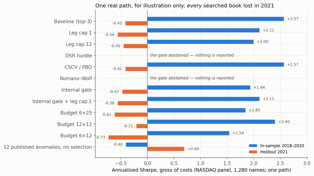
I gave a research agent four years of prices with no predictable structure in them — none, by construction — and it came back with a long/short book, an in-sample Sharpe of 2.1, and a paragraph explaining the economics of an effect that does not exist.

That is the measurement in this post. The more useful result is the second one: 88% of that number is accounted for by two integers — how many backtests the agent ran, and how many of the winners it blended into the book it reported. Only one of those is in the log everybody proposes to collect.

This closes a sequence. In August, having built an agentic research pipeline in May and measured a 2× lift in hypotheses tested per week, I priced a risk I had not thought to price: independent research runs against the same model produce books correlated at 0.62, a crowding exposure that appears in nobody’s risk report. That post ended with a claim I stated and did not measure — that faster hypothesis generation makes overfitting worse rather than better. This is the measurement, and my pre-registered prediction about how it would come out was wrong.

The one property agentic research has that human research never had

Every multiple-testing correction in finance founders on the same rock: you cannot observe the denominator. Harvey, Liu and Zhu built their t-statistic hurdle on an estimate of how many factors had been tried across the profession, not how many were published [1]. Harvey’s 2017 AFA presidential address is largely an argument about unreported trials [2]. The Deflated Sharpe Ratio requires you to supply the number of trials, and its authors are candid that in practice you are guessing [3]. Each method asks the researcher a question the researcher cannot honestly answer: how many things did you try before this one?

An agentic pipeline is different in exactly one respect. It has to ask the harness for every backtest it runs. The trial count is not a memory or an act of professional honesty. It is a log file.

So I built a minimal research agent, gave it one tool, recorded everything, and checked what the log is worth. The short answer is that it is worth less than I expected, for a reason that turns out to be measurable and fixable.

Setup

The harness. One command: submit up to 25 expressions, receive their in-sample scores. At most 12 such calls. The agent never sees prices, dates, tickers, or the holdout — the panel is anonymised to integer asset IDs and an integer time index, and the holdout files were physically absent from the filesystem while the runs executed. Every submission is logged with a timestamp, alongside a one-line hypothesis per batch and a free-text journal. The run ends when the agent reports exactly three signals.

What a “book” is, and the two counts that matter. Every arm’s output is scored the same way: three signals, equal-weighted into one book. The pre-registered primary rule takes the three highest-scoring signals a run evaluated, not the three it chose to report — the gap between the two is small and is itself reported below. N is the number of trials in the log. k is the number of additive legs in the resulting book: three for a searcher whose signals are single expressions, more for one whose signals are themselves sums. Those two integers carry the whole argument.

The signal language. A small price-only grammar: returns, moving averages, rolling moments, range position, rolling beta and correlation to the equal-weight panel, plus cross-sectional and time-series normalisations and arithmetic. It is the grammar from the August post, which matters — it was fixed before this hypothesis existed. Each signal becomes a dollar-neutral, rank-weighted long/short book with a one-day implementation lag.

The comparison arms. Three mechanical arms plus a no-selection placebo. The two that search run at the agent’s interaction schedule — 12 rounds of 25 candidates, feedback once per round. Matching rounds rather than evaluations is deliberate: in adaptive data analysis the damage scales with how many times you look and act, not with the raw query count [4].

Arm	What it is
AGENT	The LLM researcher above
OPT	Evolutionary search over the same grammar, at three selection pressures (soft, medium, hard — how aggressively each generation is bred from the current leaders)
CANON-SAMPLER	Canon-shaped expressions with jittered parameters, no feedback — prior direction without optimisation
CANON placebo	Twelve published anomalies in the same grammar, no selection at all

The data. The primary setting is synthetic: factor-structured panels with regime-switching volatility and fat tails, and zero predictability by construction. Volatility is forecastable; returns are not. The true Sharpe of every signal is zero, so every point of in-sample Sharpe is selection, and I can generate independent panels at will. The second setting is the real NASDAQ panel from the August post — 1,280 names, 2018–2023, train through 2021, holdout 2022 to May 2023.

The analysis plan, estimators, inclusion rule and predictions were committed to git before the first agent run. The repo holds the commit history, every harness log with its batch notes and research journals, a manifest of all 227 attempted runs including the five abandoned and why, and a list of every deviation from the plan.

1. What a research agent does with data that contains nothing

Twelve independent zero-alpha panels, one agent run each, identical prompt to the real-panel runs.

Every run found something. Every run wrote a confident rationale. From the report of a run on a panel whose returns are serially unpredictable by construction:

“All three combine the two independently validated engines: long-horizon cross-sectional mean reversion (ma 120-250, plateau confirmed across ret, ma, minr and maxr formulations at horizons 60-250) and a weekly return echo (returns from days t-8 to t-5 predict positively, with a coherent oscillating lag profile).”

There is no echo. There is no reversal. There is nothing.

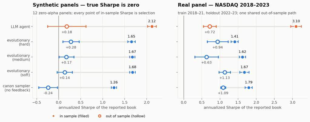
Zero-alpha panels	Reported in-sample Sharpe	Realised out-of-sample Sharpe
LLM agent (12 runs)	2.12 (SE 0.10)	+0.18 (SE 0.44)
Evolutionary, soft (12 panels)	1.68 (SE 0.07)	+0.14 (SE 0.24)
Evolutionary, medium	1.67 (SE 0.05)	+0.17 (SE 0.22)
Evolutionary, hard	1.65 (SE 0.11)	+0.28 (SE 0.22)
Canon sampler, no feedback	1.26 (SE 0.08)	−0.24 (SE 0.29)

The reported book is the equal-weight composite of the three highest-scoring signals a run evaluated — the pre-registered primary rule, which is why it differs slightly from what the agent chose to report. True out-of-sample Sharpe is zero for every arm by construction, and every row is consistent with that. Standard errors are across panels.

A Sharpe ratio of 2.12, in-sample, on a book, over four years of daily data, from a panel with no signal in it.

A little over half of that is textbook. The expected maximum Sharpe of a single expression over the agent’s own median 146 logged trials is 1.15 (SE 0.03, across the twelve panels’ random-expression pools) — the expected-maximum-Sharpe effect [3], computed here as the exact order statistic over an empirical null pool drawn from the same grammar. That accounts for 54% of the 2.12. Note what the benchmark cannot do: those are single expressions, and it takes a single expression as the answer. Hold that thought — the missing 0.97 is the subject of section 3.

The agent’s own judgment is not the problem. It usually declines to report its top three by raw score, preferring what it calls “plateau” specifications; that restraint moves the number by 0.03 (2.08 chosen versus 2.12 argmax).

In-sample versus out-of-sample by search arm

2. It manufactures more than a machine built to overfit

Paired by panel, against the evolutionary optimiser at the identical interaction schedule, using only the twelve primary runs:

Contrast, in-sample Sharpe (12 paired panels)	Difference	SE	t
Agent − evolutionary (soft)	+0.44	0.11	+3.9
Agent − evolutionary (medium)	+0.45	0.11	+4.1
Agent − evolutionary (hard)	+0.46	0.09	+5.2

On the real panel the gap is larger: 3.10 against 1.41–1.67.

That is the in-sample difference, and it is solid. The out-of-sample differences are not: those contrasts carry standard errors of 0.35 to 0.42, against a minimum detectable effect of about 1.0 Sharpe, and the pre-registered block bootstrap on the real panel returns a 95% interval of [−0.53, +1.99] for the agent’s realised Sharpe alone. Nothing in this study establishes that the agent’s books perform worse out of sample than a mechanical optimiser’s. What it establishes is that at a matched interaction budget, the agent converts noise into reported Sharpe more efficiently.

My pre-registered prediction was the opposite — that the model’s priors would act as a regulariser, keeping it in the published canon rather than in the noise, so it would overfit less. Wrong, at t ≈ 4.

3. Where the extra Sharpe comes from is not more searching

The mechanism is in the logs, and it is not model priors.

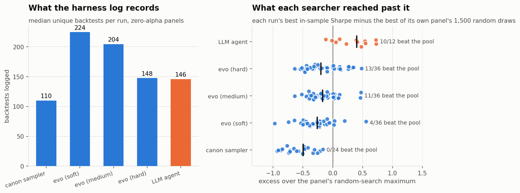
The agent logs a median of 146 unique backtests per zero-alpha run, against 148–225 for the evolutionary arms: level with the hardest setting, well below the softer ones. It is not searching harder — and note that the largest gap in the table above, +0.46, is against the arm that runs the same number of trials.

The difference is in what gets reported. Every run reports three signals, which are equal-weighted into one book. For the mechanical arms each of those three is a single expression, so the book has 3 legs. The agent’s three are themselves sums: a median of 4.2 legs each on zero-alpha panels, so its book carries about 12.5. That is the second integer, and no trial-count correction records it.

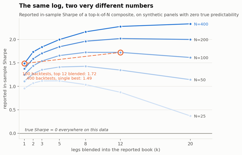
To isolate it I ran a controlled experiment on the zero-alpha panels with no agent involved: draw N random expressions, keep the top k by in-sample Sharpe, equal-weight them into a book, and record what the book reports.

Moving between curves is the familiar overfitting-versus-trials axis. Moving right along a curve is the aggregation axis nobody logs. The two trade off against each other: a pipeline that logs 100 backtests and blends its top 12 reports 1.72, while one that logs 400 and reports a single best reports 1.49. No alpha in either case, and the first pipeline’s log looks four times cleaner.

The arithmetic is standard portfolio algebra pointed at noise. Selecting k signals on in-sample performance and averaging them keeps the selected mean and cuts the variance — but the legs are not independent, so the gain is √(k / (1 + (k−1)ρ̄)), not √k. Fitting that form column by column over the monotone region gives ρ̄ of 0.41–0.47 at the trial counts that matter here, a ceiling of about 1.5× however many legs you add. That is why the curves flatten. They turn down at small N for a different reason: once k is a large fraction of N you are averaging in candidates that were barely selected at all. Novy-Marx made the combination point for strategies built from multiple signals and derived corrected critical values for it [5]; what is new here is an agent that was never asked to combine anything doing it unprompted, and the interchangeability of the two axes at a fixed log.

The closure. Take each run’s own logged trial count and its own book leg count, look up what blind top-k-of-N selection produces at that point on the surface, and compare:

Arm	Median trials	Legs in book	Blind top-k-of-N predicts	Actually reported	Residual
LLM agent	146	12.5	1.86	2.12	+0.26
Evolutionary, hard	148	3	1.68	1.65	−0.03
Evolutionary, medium	205	3	1.73	1.67	−0.05
Evolutionary, soft	225	3	1.77	1.68	−0.09
Canon sampler	110	3	1.56	1.26	−0.31

Two integers and no model price the evolutionary arms to within 0.09, and account for 88% of the agent’s number. The residual is +0.26 (t ≈ 2.1 once the surface’s own estimation error is propagated) — small next to the 1.86 that blind selection explains. And the leg axis alone carries most of the agent’s edge over the mechanical searchers: holding trials at the agent’s own 146 and moving the book from 3 legs to 12.5 adds +0.25, against a measured agent-minus-mechanical gap of +0.45.

So the agent beats the optimiser and is beaten by blind selection at its own operating point, and both facts have one cause. It blends; they do not.

That also settles what happened to the estimator I pre-registered. I had planned to report an effective trial count — the random draws from this grammar needed to match a run’s best score. It cannot be computed for most agent runs: 10 of 12 exceed the best their own panel’s 1,500-draw random pool reached, so no trial count reproduces them. That is partly a property of a finite pool and it is not agent-specific — 13 of 36 hard evolutionary runs also clear their pool — so nothing here rests on it. The direction is informative, though: a deeper random-expression pool (depth 6, mean complexity 5.9 against the shallow pool’s 3.6) lifts the 99th percentile from 0.95 to 1.24 and the maximum to 1.79 without closing the gap, because random expressions almost never build composites — mean legs 1.15.

Depth is not the axis. Blending is.

What the log records versus what random search reaches

4. The real panel

Six agent runs on the NASDAQ panel, trained through 2021, scored on 2022 to May 2023.

Real panel	Train	Holdout	Legs in book	Daily turnover
LLM agent (6)	3.10 (SE 0.15)	+0.72 (SE 0.18)	6.0	0.24
Canon sampler (5)	1.79 (SE 0.10)	+1.09 (SE 0.07)	3	0.45
Evolutionary, soft (5)	1.67 (SE 0.13)	+1.13 (SE 0.16)	3	0.43
Evolutionary, medium (5)	1.62 (SE 0.09)	+0.63 (SE 0.32)	3	0.26
Evolutionary, hard (5)	1.41 (SE 0.10)	+0.94 (SE 0.29)	3	0.49
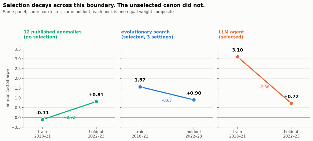
12 published anomalies, no selection	−0.11	+0.81	—	0.14

The last row is the control that makes the rest interpretable, and it is scored exactly like every other row — one equal-weight composite, same backtester, same holdout — with no selection applied. It does not decay across this boundary. It improves, from −0.11 to +0.81. The 2022–23 environment was kinder to these exposures on this universe than the training window was.

So the regime component of the agent’s decay is not merely small; it is negative. The control licenses one claim and not a stronger one: the unselected canon did not decay here, so the regime cannot explain the agent’s 2.4-point gap. It does not follow that selection explains all of it — the canon composite is loaded the opposite way from a book selected to score 3.10 in the training window, and the pre-registered random-search leg that would have measured the selection component directly was not run.

Note what the ordering does not do. It is not monotone — the medium evolutionary arm has the lowest holdout Sharpe of any arm, below the agent’s — and every one of those holdout differences sits inside the block-bootstrap intervals. The real panel cannot adjudicate between these arms.

Turnover does not explain the gap either: the agent’s books turn over 24% of gross per day, at the low end of the arms rather than the high end.

The unselected canon did not decay across this boundary

5. What the number is worth, and what it is not

The obvious next move is to use the zero-alpha number as a correction: subtract what the pipeline manufactures from noise off the face value of what it reports on real data. Since true Sharpe on the synthetic panels is zero by construction, the manufactured component is the reported in-sample Sharpe itself — 2.12 for the agent. That gives 3.10 − 2.12 = 0.98 predicted against 0.72 realised, which looks like a hit.

It is not. Run the same arithmetic for every arm:

Arm	Zero-alpha manufacture	Real face	Predicted	Realised	Predicted − realised
LLM agent	2.12	3.10	0.98	0.72	+0.26
Evolutionary, soft	1.68	1.67	−0.00	1.13	−1.13
Evolutionary, medium	1.67	1.62	−0.05	0.63	−0.68
Evolutionary, hard	1.65	1.41	−0.25	0.94	−1.18
Canon sampler	1.26	1.79	0.54	1.09	−0.55

A negative last column means the haircut left too little on the table. Mean error −0.66. The correction under-predicts realised performance in four arms out of five, and the agent’s near-miss is the one that landed the other way. These are five books on one shared holdout path, not five independent draws, so this is one observation with five views of it rather than five tests. The reason is in the previous table: this holdout carried a tailwind of roughly +0.9 for canonical exposures, which a calibration built on noise cannot know about.

So the zero-alpha number measures how much in-sample Sharpe your pipeline manufactures from nothing. It is not a forecast of out-of-sample performance, because realised performance also contains whatever the regime does to your exposures, and that term is not small. What it is worth is the overstatement:

Selection overstatement — $100M book at 10% target volatility
Face in-sample Sharpe of the reported book	3.1
Measured manufacturing capacity (zero-alpha calibration)	2.1
Annual return overstatement	≈ $21M
In basis points of notional	≈ 2,100 bp

The amount by which the in-sample report overstates, measured on data containing no alpha. Gross of costs, rounded. Not a forecast and not strategy P&L: the row above shows the haircut does not predict realised returns. Absolute performance levels on a survivorship-conditioned panel are not defensible and no such claim is made.

Things that did not work

Two pre-registered predictions failed. The first, above: the prior did not act as a regulariser. The second concerned the planted-alpha panels, where I buried two effects of equal calibrated in-sample strength — one canon-shaped (short-horizon reversal), one deliberately anti-canon (a kurtosis effect the literature points away from) — expecting the agent to find the canon-shaped one better and the mechanical arms to show no such asymmetry. Both halves were wrong. At the higher plant strength the agent captured the anti-canon plant better (0.50 versus 0.41), and it was the evolutionary arm that showed the large asymmetry (0.87 versus −0.02) and delivered more of the real alpha out of sample (1.15 versus 0.50). The comparison is confounded — the plants were matched on in-sample strength, but their oracle holdout Sharpes came out at 0.46 and 1.30 — and the agent contributes four runs per cell.

A metric that dissolved against its null — for the second post running. Regressing the agent’s real-panel books on the twelve-anomaly basis gives a mean R² of 0.50: the agent is largely reproducing published anomalies. Run the same regression on random expressions from the same grammar and you get 0.72. Noise projects onto the canon basis better than the agent’s books do — so the metric ranks the agent as less canonical than random noise, which is not a statement about the agent at all. It measures the dimensionality of price-signal space. The lesson is cheap and general: any spanning statistic needs a null drawn from the same generator, or it is measuring the basis.

The look-ahead screen cannot fire. The holdout sits inside the model’s training corpus, so I pre-registered a one-sided screen against block-bootstrap continuations of the training panel — futures the model cannot have seen. Resampling training returns reproduces the structure the books were selected on, so the synthetic benchmark runs at 1.5–2.0 Sharpe for selected books and the statistic is negative by construction (Δ = −0.92; −1.64 under the demeaned variant). It found no evidence of pretraining leakage; it also could not have. The construction is in the repo.

The model changed underneath the experiment. Two-thirds of the way through, a rate limit forced a checkpoint switch. Four partly-completed runs were abandoned under the pre-registered inclusion rule and re-run on the same four panels; a fifth run was abandoned after I contaminated it with an operator timing probe. All five are in the manifest. The twelve primary zero-alpha runs are all on the first checkpoint. Three bridge runs on the second checkpoint over the same panels reported 2.74 against 2.09 for the first checkpoint on those panels. That gap is not identified, by this post’s own mechanism: the bridge runs used their full 300-trial budget against the primary runs’ ~145, and at fixed leg count the surface predicts about half of the 0.65 gap from trials alone. Three runs is an anecdote in any case; it is reported because it is the clearest available evidence that these numbers are a snapshot of specific checkpoints. Which checkpoint served each run was never recorded — it is reconstructed from run identifiers and timing, which is a defect in my instrumentation and is flagged in the repo.

What this does and does not show

It does not show that agent-generated books underperform mechanically-generated ones out of sample. Those contrasts are inside their standard errors and the design cannot resolve them.

It does not show that a zero-alpha haircut predicts realised performance. Section 5 shows it does not.

The limitations that matter, in order. This is a minimal single-loop researcher — one agent, one tool, ≤300 trials, no holdout gate, no research committee — one to two orders below a production pipeline, and everything a real stack adds either raises the trial count or is a control whose value this same instrumentation would demonstrate. It is a floor. One model family, and a checkpoint that changed mid-study; the cross-family experiment could not be run. The real panel is one shared out-of-sample path on a survivorship-conditioned universe inside the model’s training corpus, so every real-panel number here is descriptive and the inference lives in the synthetic arm. Twelve panels is a small cross-section and every interval is wide. And the mechanical arms are matched on rounds and grammar but not perfectly: the evolutionary arm is seeded and mutated at bounded expression depth while the agent writes free-form strings, so the agent searches a strictly larger subspace — which is consistent with the finding, since composite depth is exactly the axis that matters, but it means “same grammar” is doing less work than it sounds like.

Eleven deviations from the pre-registration — the censored trial-count estimator, the random-search decomposition leg that was not run, 60 continuations instead of 200, the warm-start evaluation basis, a prompt revised after the plan was committed, and the rest — are listed in DEVIATIONS.md.

So what do you do

Build the surface for your own stack. This is the differentiated move and it costs almost nothing. Construct a panel matched to your universe — same factor covariance, same volatility dynamics, same fat tails — with the conditional mean stripped out, and verify the construction by checking that an oracle signal earns zero. Then run your own pipeline against it, unmodified, and record what it reports at each (trials, legs) pair you actually operate at. That grid is your pipeline’s manufacturing capacity in the units you use, and you can look up any future result on it. For the pipeline here it was 2.1 Sharpe. The generator and the surface code are in the repo and the whole thing runs on a laptop.

Log two numbers, not one. The trial count is now an artifact rather than a memory, and a pipeline that cannot produce one is worse off than this toy. But on its own it prices nothing: a 12-leg book from 100 trials carries more selection than a single expression from 400, and only the first of those facts is in the log everyone proposes to keep. With both numbers you can look the answer up on your own surface. With one you cannot.

Then subtract, and stop there. The result tells you how much of the reported number is manufacturing. It does not tell you what the book will earn, because that also depends on what the regime does to your exposures — and section 5 shows that term is larger than the correction.

Every zero-alpha run in this study produced a good economic story — volatility term structure, lottery preference, reversal at horizons where reversal is documented — attached to nothing. The pipeline is a fine instrument. It is also, on data containing nothing, a machine for producing a Sharpe of 2.1 and a paragraph about why.

Code and data

Repo: jkinlay/agent-selection-surface

The repository contains the pre-registered analysis plan committed before the first run, a deviations list, the frozen prompt, the harness, the mechanical arms, the synthetic generator with its calibration constants, every run log with its batch notes and research journals, the manifest of all 227 attempted runs with dispositions and reasons, the backtester canary tests, and the analysis and figure code. Everything downstream of the LLM calls reproduces from seeds; the LLM calls are not re-runnable, which is why the logs are included in full.

Two requests of anyone re-running it. Run the zero-alpha arm first — it is what makes every subsequent number interpretable. And log the leg count, not just the trial count.

References

[1] Harvey, Liu & Zhu, …and the Cross-Section of Expected Returns, Review of Financial Studies 29(1), 2016.

[2] Harvey, Presidential Address: The Scientific Outlook in Financial Economics, Journal of Finance 72(4), 2017.

[3] Bailey & López de Prado, The Deflated Sharpe Ratio, Journal of Portfolio Management 40(5), 2014; Bailey, Borwein, López de Prado & Zhu, Pseudo-Mathematics and Financial Charlatanism, Notices of the AMS 61(5), 2014, for the expected-maximum-Sharpe result used in section 1.

[4] Dwork, Feldman, Hardt, Pitassi, Reingold & Roth, The reusable holdout: Preserving validity in adaptive data analysis, Science 349(6248), 2015 — guarantees degrade with the number of adaptive rounds, which is why every arm here is matched on rounds rather than evaluations.

[5] Novy-Marx, Backtesting Strategies Based on Multiple Signals, NBER Working Paper 21329, 2015 — in-sample test statistics inflate with the number of combined signals, with corrected critical values. The aggregation axis in section 3 is this effect, arrived at by an agent that was not asked to combine anything.

[6] skfolio, load_nasdaq_dataset — daily adjusted closes, 1,455 NASDAQ constituents, 2018-01-02 to 2023-05-31, documented by its authors as a stale dataset not intended for investment or commercial use. Filtered here to 1,280 names with median price ≥ $5; SHA-256 of the source file is in the analysis plan.

[7] Canonical anomalies in the placebo: Jegadeesh & Titman (1993) with the Carhart (1997) 12-1 construction; Jegadeesh (1990); Ang, Hodrick, Xing & Zhang (2006); George & Hwang (2004); Frazzini & Pedersen (2014); Boyer, Mitton & Vorkink (2010); Moskowitz, Ooi & Pedersen (2012); Novy-Marx (2012). The twelfth, a 60-minus-120-day momentum-acceleration variant, is a construction of my own.

Disclosure: I run systematic strategies. Nothing here is a recommendation, and no strategy discussed is one I trade. These are diagnostic quantities from a methodological experiment on a stale public dataset, not a track record.

May 17, 2026May 17, 2026

Agentic Workflows for Alpha Research

A 12-Week Practitioner Case Study

There is by now a small mountain of vendor material claiming that AI agents will run hedge funds. The reality on the ground — for those of us who actually do the work — is more interesting and more useful. Agentic workflows, properly constructed, materially accelerate the parts of quant research that consume the most time. They also fail in specific, predictable ways that you can defend against if you take them seriously and ignore if you don’t.

This post is a write-up of an architecture I have been using for the last four months on an FX-carry research project, and what it changed about my throughput. The headline finding is that the right unit of measurement is not “ideas per hour” — which is misleading — but ideas that survive a human-grade critique per month. On that metric the lift, on this single workstream, is on the order of 2× rather than 10×, and it comes from a very specific allocation of work between the human and the agent.

The single most important thing to internalise before reading further is that the architecture is the load-bearing piece — not the prompts, not the model choice. Most of what makes this stack work would still work if you swapped Claude for any other frontier model; very little of it would work if you swapped the typed handoffs, the research log, and the human gates for a single conversational thread. The recent multi-agent literature converges on the same conclusion from the software-engineering side — AutoGen [1] frames LLM applications as configurable agents with structured interaction, and MetaGPT [2] argues explicitly that encoding standard operating procedures into role-specialised pipelines is what produces reliable outputs. The point of this post is to make the same argument for the quant-research side, and to instrument the claim with measured numbers rather than vibes.

1. What alpha research actually consists of

Before discussing what to automate, it helps to be honest about what the day-to-day is.

A reasonable decomposition of the time I spend on a single research idea, end-to-end:

Literature triage and replication — finding the three papers that matter out of the thirty that cite the relevant phenomenon, and reproducing their core result. 20–25%.
Hypothesis specification — stating the economic claim precisely enough that a backtest can falsify it. 5%.
Data wrangling — sourcing, aligning, point-in-time correctness, handling holidays and corporate actions. 25–30%.
Implementation — writing the signal, the portfolio construction, the cost model, the evaluator. 10–15%.
Diagnostic and ablation work — by-regime, by-subsample, by-feature, transaction-cost sensitivity, parameter stability. 20%.
Judgment and synthesis — deciding whether what you have is real, whether it adds to the existing book, and whether to risk it. 10%.

The last category is the one that actually distinguishes a senior researcher from a junior one, and it is the category that AI agents are worst at. The first four are the categories where they are dramatically better than the alternative of doing it yourself.

The architecture I will describe is built around that asymmetry: aggressively delegate the first four, keep judgment human, and instrument the boundary between the two so failures are visible early.

2. The naive loop and why it fails

The seductive thing to do — and the thing every demo on Twitter shows — is to wire a single capable LLM up to a Python sandbox and a price-history database and tell it “find me alpha in EM FX”. I tried this. So has everyone.

What you get back, reliably, is a strategy with an in-sample Sharpe of 2.4 that does the following four things:

Uses some flavour of recent-return signal with a lookback chosen to fit the sample.
Sizes positions inversely proportional to realised volatility, with the volatility window also chosen to fit the sample.
Quietly references a feature whose construction has a one-step look-ahead bug.
Reports backtest statistics over a period that conveniently excludes the 2022 carry drawdown.

The agent is not malicious. It is doing exactly what you asked. The objective you wrote — “maximise Sharpe on this dataframe” — has no concept of out-of-sample, of economic prior, or of regime. An agent with code execution and a permissive objective is a specification-gaming machine, and the result is the alpha-research equivalent of a model that achieves 99% accuracy on MNIST by memorising the test set.

This is a textbook case of the failure modes formalised in Amodei et al. [3]: reward hacking when the objective is misspecified, distributional shift between training and deployment regimes, and absence of scalable supervision when the supervisor is the same LLM doing the optimisation. The lesson is that the single-agent, single-objective loop is the wrong abstraction. Quant research has more than one objective, and the objectives are partly adversarial.

3. The architecture: separated roles, instrumented handoffs

The setup that has worked for me has four roles, each instantiated as a separate LLM call with its own system prompt, tool access, and — importantly — its own context window. They communicate via a structured research-log database rather than by sharing memory directly.

Proposer. Reads recent literature and the current research log, and emits a single falsifiable hypothesis in a fixed schema: economic claim, dependent variable, predictor(s), sample, null. No code. Read access to a curated paper corpus and to the research log; no access to price data. Forcing the hypothesis through a schema is the single most important constraint in the whole stack — it makes “interesting-sounding but unfalsifiable” outputs impossible.

Implementer. Takes a single approved hypothesis and produces a notebook that tests it. Has read access to data and write access to a sandboxed compute environment. Critically, has no access to the results of prior implementations — this prevents the agent from anchoring on prior backtest numbers and tuning the new implementation to match.

Critic. Reads only the implementer’s notebook and its output. Its prompt is to produce an adversarial list of reasons the result might be spurious: look-ahead bugs, multiple-testing inflation, regime cherry-picking, cost-model optimism, feature contamination. Outputs a checklist with severity. The Critic does not get to fix anything; it only files findings.

Replicator. Takes the Critic’s findings and the original notebook and produces a panel of robustness tests: alternative samples, alternative cost assumptions, leave-one-out by feature, and deliberate ablations of any flagged components. Outputs a single comparison table.

Replicator independence at promotion stage. For any candidate that has cleared the Critic and is being considered for the second human gate, the Replicator is not allowed to reuse the Implementer’s feature-generation code. It receives only the hypothesis schema and a frozen data contract, and reimplements the signal independently. This turns the Replicator from a robustness-script generator into a genuine independent check, and catches at least one class of bug — silent feature-construction errors — that the Critic structurally cannot detect from reading the Implementer’s notebook alone.

The human (me) sits as a gate at two points: between Proposer and Implementer (does this hypothesis deserve compute?) and between Replicator and “promotion to candidate” (is the robustness panel convincing?). Everything in between runs without supervision.

What this is, and what it is not. The stack is autonomous only inside pre-specified rails. It is a controlled batch pipeline with LLM modules, not an autonomous research scientist. It does not choose its own data permissions, change its own validation criteria, redefine the promotion threshold, or promote its own results. That is by design — and it is the design feature that separates this from the “AI hedge fund” pitch. The fully autonomous research agent is, as far as I can tell, not yet a viable target; what is a viable target is making each non-judgment step of the research pipeline an order of magnitude cheaper, while leaving the judgment steps untouched.

The key invariant is that no role sees its own prior outputs as ground truth. Each handoff is a fresh context with the schema-typed artifact and nothing else. This is what kills the most common failure mode of single-agent loops, which is that the agent quietly accumulates evidence in favour of its earlier guesses.

Schematically:

                   ┌──────────────────────┐
                   │  Research-log DB     │
                   │  (typed artifacts)   │
                   └─────────┬────────────┘
                             │
   ┌─────────┐   hypothesis  │   notebook   ┌────────┐
   │Proposer ├───────────────┴──────────────┤Impl.   │
   └────┬────┘            ▲                 └───┬────┘
        │                 │                     │
     human gate           │                     │
        │                 │   findings          ▼
        │             ┌───┴────┐           ┌────────┐
        └────────────►│Critic  │◄──────────┤notebook│
                      └───┬────┘           │+ output│
                          │                └────────┘
                       robustness
                          ▼
                      ┌──────────┐
                      │Replicator│──► comparison table ──► human gate
                      └──────────┘

4. The objective function, written down

It is worth being explicit about what the system as a whole is optimising. A single Sharpe number is not it. The composite I use is:

U \;=\; \mathrm{IR}_{\text{oos}} \;-\; \lambda_1 \,\big|\mathrm{IR}_{\text{is}} – \mathrm{IR}_{\text{oos}}\big| \;-\; \lambda_2 \, k_{\text{eff}} \;-\; \lambda_3 \, S_{\text{tc}} \;-\; \lambda_4 \log\!\big(1 + N_{\text{trials}}\big) \;-\; \lambda_5 \, C_{\text{frag}}

Term by term:

Out-of-sample IR. The information ratio of the strategy on data the Implementer has not seen. The sample boundary is fixed by the Proposer in the hypothesis schema, not chosen by the Implementer.
Overfitting drift. The absolute gap between in-sample and out-of-sample IR. A strategy with a 2.0 in-sample IR and 0.4 out-of-sample IR is worse than one at 0.9 / 0.7. The penalty weight is calibrated ex ante and frozen before any candidate is evaluated.
Effective parameters, k-eff. A degrees-of-freedom proxy that counts lookback choices, thresholds, feature inclusions, regime switches, and any other knob whose value was set after seeing data. The count is generated by the Implementer at submission time as part of the notebook schema, not estimated post hoc. A strategy with three tuned knobs is preferred over an empirically-equal strategy with eleven.
Transaction-cost sensitivity, S-tc. The slope of net returns with respect to a 1 bp shift in assumed cost. A strategy that goes from a 0.8 IR at 2 bps assumed cost to 0.0 at 3 bps is fragile to a part of the world we do not know well, and the objective should say so.
Search-intensity penalty. A logarithmic penalty in the effective number of trials the stack has run on related hypotheses in the same workstream. This is the term that explicitly links the objective to the multiple-testing literature: White’s Reality Check [4] on data-snooping, Bailey, Borwein, López de Prado and Zhu [5] on the probability of backtest overfitting (which gives a usable Deflated Sharpe Ratio formulation), and Harvey, Liu and Zhu [6] on inflated significance in factor research. Without it, an agentic stack that runs 38 hypotheses in 12 weeks will mechanically look better than a human who runs 11, even when the marginal hypothesis is no better — exactly the dynamic those papers warn against. The effective trial count is incremented every time the Implementer commits a notebook touching the same dependent variable, regardless of whether the result is positive.
Fragility penalty, C-frag. Captures dependence on one date range, one currency, one regime, one cost assumption, or one feature family. Computed as the maximum proportional loss in IR when any single such dimension is ablated. A strategy whose IR collapses when 2022 is excluded scores poorly regardless of headline performance.

The Proposer, Implementer, and Critic all see this composite. The Implementer is not told to maximise it — that would re-introduce the specification-gaming problem. It is told to test the hypothesis. The composite is used by the Critic to flag any result where any term contributes negatively beyond a fixed threshold, and by the human gate to compare candidates.

This is the same idea that underlies penalised regression: you write your taste explicitly into the objective rather than relying on the optimiser to share it. The λ weights are not magic; they are chosen so that — on a held-out historical set of strategies whose ex-post five-year outcomes are known — the ranking produced by U correlates with realised forward performance. The calibration is done once, before any candidate from the current workstream is evaluated, and is not re-tuned during the run.

5. The tooling, concretely

For practitioners who want to assemble something equivalent, the components I am using:

LLM: Claude Opus for Proposer and Critic (better at synthesis, more skeptical reading); Claude Sonnet for Implementer and Replicator (faster, sufficient for code). All calls go through the standard Anthropic SDK with prompt caching on the role system prompts — this matters for cost, since the role prompts are long and reused on every turn.
Execution sandbox: a pinned Docker image with pandas, numpy, statsmodels, scikit-learn, and a vendored copy of the data layer. No network. The sandbox is rebuilt nightly to keep dependencies fresh; the image hash is stored in every research-log entry so any result is exactly reproducible.
Research-log DB: SQLite with five tables — hypotheses, implementations, results, critiques, robustness. Every artifact has a UUID, a parent UUID, a timestamp, the image hash of the sandbox at the time, and the git commit of the data layer. This is the single most-valuable component and the one most people skip.
Data layer: a thin wrapper over the price store that enforces point-in-time correctness by construction. Any access by date t can only return data available at or before t. The wrapper raises if asked for anything later. This single guardrail prevents the most common look-ahead bug.
Human-gate UI: a tiny Streamlit app that surfaces (hypothesis, notebook, critique, robustness) as a single page with approve / reject / send-back-with-comment buttons. The friction here matters; if the gate is cumbersome you start waving things through.

A simplified version of the Proposer call, just to make it concrete:

# proposer.py
import anthropic, json
from research_log import recent_hypotheses, recent_critiques

client = anthropic.Anthropic()

SYSTEM = """You are the Proposer in a four-role alpha-research loop.
You produce ONE testable hypothesis in the schema below. You do not
write code. You do not run backtests. You do not propose hypotheses
that have been tested in the last 60 days (see prior list).

Schema (JSON):
{
  "economic_claim":      str,   # one sentence, mechanism stated
  "dependent_variable":  str,   # what we're trying to predict
  "predictor":           str,   # the signal, defined precisely
  "sample":              str,   # universe + date range, including OOS
  "null":                str    # what would falsify the claim
}

Rejection criteria you must apply to your own output before emitting:
- If the mechanism is "factor X has predicted Y" with no economic
  story, reject and try again.
- If the predictor's definition references information that would
  not have been available at decision time, reject and try again.
- If the sample omits a regime the claim should hold in, reject
  and try again.
"""

def propose(literature_excerpts: list[str]) -> dict:
    user_msg = {
        "recent_hypotheses": recent_hypotheses(days=60),
        "recent_critiques":  recent_critiques(days=60),
        "literature":        literature_excerpts,
    }
    resp = client.messages.create(
        model="claude-opus-4-7",
        system=[{"type": "text", "text": SYSTEM,
                 "cache_control": {"type": "ephemeral"}}],
        max_tokens=1024,
        messages=[{"role": "user",
                   "content": json.dumps(user_msg)}],
    )
    return json.loads(resp.content[0].text)

The Critic and Replicator are structurally similar — different system prompts, different tool access, same JSON-in / JSON-out discipline. The full set of prompts is on my GitHub; I will not paste all four here because the post would double in length and the prompts are not the load-bearing piece.

6. Validating the Critic

The Critic is a control on the rest of the pipeline. A reader is entitled to ask how I know it works, since using one LLM to validate another LLM’s output is exactly the circularity Amodei et al. [3] flag under scalable supervision.

The answer is a small but explicit validation suite. I seeded 25 notebooks with known defects across six categories: one-step look-ahead in a feature, sample-boundary drift, omitted transaction cost, regime cherry-picking, an unstable to-be-tuned parameter, and silent feature-name collision. Each defect was injected at a severity calibrated to a plausible human error, not an obvious one. The Critic was run blind on each notebook, alongside 25 syntactically-similar clean controls.

Defect class	Seeded	Caught	Missed	False positives (on clean controls)
Look-ahead	5	5	0	0
Sample-boundary drift	5	4	1	1
Cost omission	5	5	0	0
Regime cherry-picking	5	3	2	2
Unstable parameter	3	2	1	1
Feature-name collision	2	1	1	0
Total	25	20	5	4

An 80% catch rate on its own is not good enough — five missed severe defects across 25 notebooks would, if unaddressed, ship five strategies built on broken foundations. That is why the point-in-time data wrapper, the Implementer’s feature-schema requirement, the Replicator’s independent reimplementation, and the human gate exist alongside the Critic. Each catches a different defect class, and the failures are largely uncorrelated. The validation exercise is repeated whenever the Critic’s prompt is materially changed.

Two caveats. First, this exercise probably understates real-world false-positive rates, because syntactically-clean controls do not have the idiosyncrasies of real notebooks. Second, it does not test the most dangerous failure mode (confidently wrong synthesis); that is governed by the quote-the-cell-output constraint discussed in §8.

7. What it changed: 12 weeks on FX carry

Before the numbers, the operational definition of “promoted to candidate” — the endpoint that does the work in the table below. A candidate is a strategy that has cleared all of the following gates:

Positive net-of-cost out-of-sample IR over the full Proposer-defined sample.
No unresolved severe finding from the Critic (severity-1 issues must be fixed and re-run; severity-2 issues must be explicitly waived in writing with reasoning).
Stable sign of IR in at least six of the eight rows of the Replicator’s robustness panel.
No single regime contributes more than 40% of total backtest P&L.
Independent reimplementation by the Replicator (see §3) produces an IR within ±15% of the original.
A human-written one-paragraph economic rationale that the candidate’s mechanism is plausible, written before viewing the final composite-U score.

A candidate is not a deployed strategy. It is a strategy that has earned the right to a further month of paper trading and live-data review before being considered for any risk allocation. In the period under discussion, neither of the two candidates has yet been promoted to risk; that is a separate decision on a separate timescale.

I ran this stack against an FX-carry research workstream from late January through mid-April 2026, alongside a personal baseline of comparable hours from the equivalent period in 2025. The work was on conditional carry — under what regimes does the standard high-minus-low carry portfolio in G10 actually pay, and can we identify the regime ex ante.

Metric	Baseline (2025)	Agentic stack (2026)	Ratio
Hypotheses formally tested	11	38	3.5×
Time from hypothesis to first backtest	~2 days	~3 hours	~5×
Hypotheses that survived Critic	n/a	14 of 38 (37%)	—
Survived robustness panel	n/a	4 of 14 (29%)	—
Promoted to candidate (human gate)	1	2	2×
Researcher hours / week	~22	~18	0.8×
API spend / week (USD)	~0	~$340	—
Sandbox compute / week (USD)	~$15	~$25	1.7×

Measurement caveats. The comparison is not a randomised productivity experiment. It is a within-person case study with obvious confounds: different calendar periods, different available frontier models, possible learning effects on my part, a different specific workstream, and a subjective promotion threshold (whose criteria are at least now written down). I report it because the direction and magnitude were large enough to matter operationally, not because it proves a general law about agentic research productivity. The 2× candidate-yield figure should be read as an order of magnitude, not a point estimate; if the same exercise produces a 1.4× or 3× result on a different workstream, I would not be surprised. The cost figures above are included so a reader can judge total spend, not just throughput — a 2× lift at 10× spend is a different proposition from 2× at 1.2×.

What the stack visibly bought me, beyond raw throughput:

More diverse hypotheses. With a low cost per hypothesis I tested several that I would normally have ruled out at the back-of-the-envelope stage. One of the two promoted candidates came from this bucket.
Better robustness coverage. The Replicator runs the same eight-row sensitivity panel on every survivor. I almost never did this by hand for marginal-looking ideas; now it is free.
Better research log. I have a typed, searchable record of 38 hypotheses, their results, their critiques, and the exact code. The log itself has caught two cases where I started to re-propose something I had already rejected.

What it did not buy me:

Better economic intuition. The Proposer’s hypotheses are competent but unsurprising; they correspond closely to what a thoughtful junior would produce. The novel angle in one of the two promoted candidates came from a conversation I had at a conference, not from the stack.
Faster judgment at the human gate. The gate took roughly the same time per candidate as before — perhaps slightly longer, because I was reviewing better-documented work.

The first of these is, I think, fundamental to the current generation of models. The second is fine — judgment should be slow.

8. Failure modes I actually saw

Three of these came up repeatedly enough to deserve naming.

Plausible-feature contamination. The Implementer would invent a feature, name it something innocuous like carry_zscore_lookback, and quietly construct it using a rolling window that included the contemporaneous observation. The Critic caught most of these. The point-in-time data wrapper caught the rest. Without both layers, I would have shipped at least one of these.

Backtest period drift. The Implementer, given freedom over the sample, would sometimes anchor the start date a few months after a known drawdown. Never the full move — that would have been obvious — but enough to materially flatter the result. The fix was to require the Proposer to fix the sample as part of the hypothesis schema, and to have the Critic flag any deviation. After this change the failure stopped.

Confident wrong synthesis. The Critic, on long notebooks, would occasionally produce a confident-sounding summary that contradicted the actual numbers in the notebook. This is the single failure mode that scared me most, because it is the hardest to catch by glance. The mitigation is to require the Critic to quote specific cell outputs verbatim in its findings, with line references. After that change, hallucinated summaries dropped to roughly zero — the constraint of having to cite a concrete output is, empirically, enough to keep the model honest.

I do not claim these are the only failure modes. They are the ones that showed up at a rate I could measure.

9. What this means in practice

If you take only one thing from this post, take this: the value of agentic workflows in quant research is mostly in the structure, not the models. The exact LLM matters at the margin. The role separation, the typed handoffs, the research log, the point-in-time data wrapper, the search-intensity term in the objective, and the human gate at the right two points — those are what convert raw model capability into research that actually deserves to be looked at twice.

The fully autonomous research agent — Proposer to deployed strategy with no human in the loop — is, as far as I can tell, not yet a viable target. The judgment step is where the value-add of the senior researcher lives, and the current generation of models is not close to substituting for it. They are close enough to substitute for the work that surrounds it, and that is a meaningful change.

What I would do if I were standing up this stack from scratch, in order:

Build the point-in-time data wrapper first. Everything downstream depends on it.
Build the research-log DB second. Typed artifacts are the single biggest determinant of quality.
Write the Proposer / Implementer / Critic / Replicator prompts third. Iterate them against your own taste; expect to rewrite them three times.
Build the Critic validation suite fourth — before relying on the Critic as a control. If you cannot measure its catch rate, you do not know what it is doing.
Build the human-gate UI last, and make it pleasant to use. If the gate is cumbersome, you will start waving things through, and the whole system collapses.

The repository accompanying this post — prompts, sandbox image, log schema, gate UI, and the seeded-defect notebook set — is at the usual place. As always, the system is set up so you can run the entire loop against the free FRED and AlphaVantage data tiers; you do not need to subscribe to anything to reproduce the structural conclusions, only the FX-carry specifics.

References

[1] Wu, Q. et al. (2023). “AutoGen: Enabling Next-Gen LLM Applications via Multi-Agent Conversation.” arXiv:2308.08155.

[2] Hong, S. et al. (2023). “MetaGPT: Meta Programming for a Multi-Agent Collaborative Framework.” arXiv:2308.00352.

[3] Amodei, D., Olah, C., Steinhardt, J., Christiano, P., Schulman, J., and Mané, D. (2016). “Concrete Problems in AI Safety.” arXiv:1606.06565.

[4] White, H. (2000). “A Reality Check for Data Snooping.” Econometrica 68(5), 1097–1126.

[5] Bailey, D. H., Borwein, J., López de Prado, M., and Zhu, Q. J. (2016). “The Probability of Backtest Overfitting.” Journal of Computational Finance 20(4), 39–69.

[6] Harvey, C. R., Liu, Y., and Zhu, H. (2016). “…and the Cross-Section of Expected Returns.” Review of Financial Studies 29(1), 5–68.

March 1, 2026March 1, 2026

State-Space Models for Market Microstructure: Can Mamba Replace Transformers in High-Frequency Finance?

In my recent piece on Kronos, I explored how foundation models trained on K-line data are reshaping time series forecasting in finance. That discussion naturally raises a follow-up question that several readers have asked: what about the architecture itself? The Transformer has dominated deep learning for sequence modeling over the past seven years, but a new class of models — State-Space Models (SSMs), particularly the Mamba architecture — is gaining serious attention. In high-frequency trading, where computational efficiency and latency are everything, the claimed O(n) versus O(n²) complexity advantage is more than academic. It’s a potential competitive edge.

Let me be clear from the outset: I’m skeptical of any claim that a new architecture will “replace” Transformers wholesale. The Transformer ecosystem is mature, well-understood, and backed by enormous engineering investment. But in the specific context of market microstructure — where we process millions of tick events, model limit order book dynamics, and make decisions in microseconds — SSMs deserve serious examination. The question isn’t whether they can replace Transformers entirely, but whether they should be part of our toolkit for certain problems.

I’ve spent the better part of two decades building trading systems that push against latency constraints. I’ve watched the industry evolve from simple linear models to gradient boosted trees to deep learning, each wave promising revolutionary improvements. Most delivered incremental gains; some fizzled entirely. What’s interesting about SSMs isn’t the theoretical promise — we’ve seen theoretical promises before — but rather the practical characteristics that might actually matter in a production trading environment. The linear scaling, the constant-time inference, the selective attention mechanism — these aren’t just academic curiosities. They’re the exact properties that could determine whether a model makes it into a production system or dies in a research notebook.

What Are State-Space Models?

To understand why SSMs have suddenly become interesting, we need to go back to the mathematical foundations — and they’re older than you might think. State-space models originated in control theory and signal processing, describing systems where an internal state evolves over time according to differential equations, with observations emitted from that state. If you’ve used a Kalman filter — and in quant finance, many of us have — you’ve already worked with a simple state-space model, even if you didn’t call it that.

The canonical continuous-time formulation is:

\[x'(t) = Ax(t) + Bu(t)\]

\[y(t) = Cx(t) + Du(t)\]

where $x(t)$ is the latent state vector, $u(t)$ is the input, $y(t)$ is the output, and $A$, $B$, $C$, $D$ are learned matrices. This looks remarkably like a Kalman filter — because it is, in essence, a nonlinear generalization of linear state estimation. The key difference from traditional time series models is that we’re learning the dynamics directly from data rather than specifying them parametrically. Instead of assuming variance follows a GARCH(1,1) process, we let the model discover what the underlying state evolution looks like.

The challenge, historically, was that computing these models was intractable for long sequences. The recurrent view requires iterating through each timestep sequentially; the convolutional view requires computing full convolutions that scale poorly. This is where the S4 model (Structured State Space Sequence) changed the game.

S4, introduced by Gu, Dao et al. (2022), brought three critical innovations. First, it used the HiPPO (High-order Polynomial Projection Operator) framework to initialize the state matrix $A$ in a way that preserves long-range dependencies. Without proper initialization, SSMs suffer from the same vanishing gradient problems as RNNs. The HiPPO matrix is specifically designed so that when the model views a sequence, it can accurately represent all historical information without exponential decay. In financial terms, this means last month’s market dynamics can influence today’s predictions — something vanilla RNNs struggle with.

Author’s Take: This is the key innovation that makes SSMs viable for finance. Without HiPPO, you’d face the same vanishing-gradient failure mode that killed RNN research for decades. The HiPPO initialization is essentially a “warm start” that encodes the mathematical insight that recent history matters more than distant history — but distant history still matters. This is perfectly aligned with how financial markets work: last quarter’s regime still influences pricing, even if less than yesterday’s moves.

HiPPO provides a theoretically grounded initialization that allows the model to remember information from thousands of timesteps ago — critical for financial time series where last week’s patterns may be relevant to today’s dynamics. The mathematical insight is that HiPPO projects the input onto a basis of orthogonal polynomials, maintaining a compressed representation of the full history. This is conceptually similar to how we’d use PCA for dimensionality reduction, except it’s learned end-to-end as part of the model’s dynamics.

Second, S4 introduced structured parameterizations that enable efficient computation via diagonalization. Rather than storing full $N \times N$ matrices where $N$ is the state dimension, S4 uses structured forms that reduce memory and compute requirements while maintaining expressiveness. The key insight is that the state transition matrix $A$ can be parameterized as a diagonal-plus-low-rank form that enables fast computation via FFT-based convolution. This is what gives S4 its computational advantage over traditional SSMs — the structured form turns the convolution from $O(L^2)$ to $O(L \log L)$.

Third, S4 discretizes the continuous-time model into a discrete-time representation suitable for implementation. The standard approach is zero-order hold (ZOH), which treats the input as constant between timesteps:

\[x_{k} = \bar{A}x_{k-1} + \bar{B}u_k\]

\[y_k = \bar{C}x_k + \bar{D}u_k\]

where $\bar{A} = e^{A\Delta t}$, $\bar{B} = (e^{A\Delta t} – I)A^{-1}B$, and similarly for $\bar{C}$ and $\bar{D}$. The bilinear transform is an alternative that can offer better frequency response in some settings:

Author’s Take: In practice, I’ve found ZOH (zero-order hold) works well for most tick-level data — it’s robust to the high-frequency microstructure noise that dominates at sub-second horizons. Bilinear can help if you’re modeling at longer horizons (minutes to hours) where you care more about capturing trend dynamics than filtering out tick-by-tick noise. This is another example of where domain knowledge beats blind architecture choices.

\[\bar{A} = (I + A\Delta t/2)(I – A\Delta t/2)^{-1}\]

Either way, the discretization bridges continuous-time system theory with discrete-time sequence modeling. The choice of discretization matters for financial applications because different discretization schemes have different frequency characteristics — bilinear transform tends to preserve low-frequency behavior better, which may be important for capturing long-term trends.

Mamba, introduced by Gu and Dao (2023) and winning best paper at ICLR 2024, added a fourth critical innovation: selective state spaces. The core insight is that not all input information is equally relevant at all times. In a financial context, during calm markets, we might want to ignore most order flow noise and focus on price levels; during a news event or volatility spike, we want to attend to everything. Mamba introduces a selection mechanism that allows the model to dynamically weigh which inputs matter:

\[s_t = \text{select}(u_t)\]

\[\bar{B}_t = \text{Linear}_B(s_t)\]

\[\bar{C}_t = \text{Linear}_C(s_t)\]

The select operation is implemented as a learned projection that determines which elements of the input to filter. This is fundamentally different from attention — rather than computing pairwise similarities between all tokens, the model learns a function that decides what information to carry forward. In practice, this means Mamba can learn to “ignore” regime-irrelevant data while attending to regime-critical signals.

This selectivity, combined with an efficient parallel scan algorithm (often called S6), gives Mamba its claimed linear-time inference while maintaining the ability to capture complex dependencies. The complexity comparison is stark: Transformers require $O(L^2)$ attention computations for sequence length $L$, while Mamba processes each token in $O(1)$ time with $O(L)$ total computation. For $L = 10,000$ ticks — a not-unreasonable window for intraday analysis — that’s $10^8$ versus $10^4$ operations per layer. The practical implication is either dramatically faster inference or the ability to process much longer sequences for the same compute budget. On modern GPUs, this translates to milliseconds versus tens of milliseconds for a forward pass — a difference that matters when you’re making hundreds of predictions per second.

Compared to RNNs like LSTMs, SSMs don’t suffer from the same sequential computation bottleneck during training. While LSTMs must process tokens one at a time (true parallelization is limited), SSMs can be computed as convolutions during training, enabling GPU parallelism. During inference, SSMs achieve the constant-time-per-token property that makes them attractive for production deployment. This is the key advantage over LSTMs — you get the sequential processing benefits of RNNs during inference with the parallel training benefits of CNNs.

Why HFT and Market Microstructure?

If you’re building trading systems, you’ve likely noticed that most machine learning approaches to finance treat the problem as either (a) predicting returns at some horizon, or (b) classifying market regimes. Neither approach explicitly models the underlying mechanism that generates prices. Market microstructure does exactly that — it models how orders arrive, how limit order books evolve, how informed traders interact with liquidity providers, and how information gets incorporated into prices. Understanding microstructure isn’t just academic — it’s the foundation of profitable execution and market-making strategies.

The data characteristics of market microstructure create unique challenges that make SSMs potentially attractive:

Scale: A single liquid equity can generate millions of messages per day across bid, ask, and depth levels. Consider a highly traded stock like Tesla or Nvidia during volatile periods — you might see 50-100 messages per second, per instrument. A typical algo trading firm’s data pipeline might ingest 50-100GB of raw tick data daily across their coverage universe. Processing this with Transformer models is expensive. The quadratic attention complexity means that doubling your context length quadruples your compute cost. With SSMs, you double context and roughly double compute — a much friendlier scaling curve. This is particularly important when you’re building models that need to see significant historical context to make predictions.

Non-stationarity: Market microstructure is inherently non-stationary. The dynamics of a limit order book during normal trading differ fundamentally from those during a market open, a regulatory halt, or a volatility auction. At market open, you have a flood of overnight orders, wide spreads, and rapid price discovery. During a halt, trading stops entirely and the book freezes. In volatility auctions, you see large price movements with reduced liquidity. Mamba’s selective mechanism is specifically designed to handle this — the model can learn to “switch off” irrelevant inputs when market conditions change. This is conceptually similar to regime-switching models in econometrics, but learned end-to-end. The model learns when to attend to order flow dynamics and when to ignore them based on learned signals.

Latency constraints: In market-making or latency-sensitive strategies, every microsecond counts. A Transformer processing a 512-token sequence might require 262,144 attention operations. Mamba processes the same sequence in roughly 512 state updates — a 500x reduction in per-token operations. While the constants differ (SSM state dimension adds overhead), the theoretical advantage is substantial. Several practitioners I’ve spoken with report sub-10ms inference times for Mamba models that would be impractical with Transformers at the same context length. For comparison, a typical market-making strategy might have a 100-microsecond latency budget for the entire decision pipeline — inference must be measured in microseconds, not milliseconds.

Long-range dependencies: Consider a statistical arbitrage strategy across 100 stocks. A regulatory announcement at 9:30 AM might affect correlations across the entire universe until midday. Capturing this requires modeling dependencies across thousands of timesteps. The HiPPO initialization in S4 and the selective mechanism in Mamba are specifically designed to maintain information flow over such horizons — something vanilla RNNs struggle with due to gradient decay. In practice, this means you can build models that truly “remember” what happened earlier in the trading session, not just what happened in the last few minutes.

There’s also a subtler point worth mentioning: the order book itself is a form of state. When you look at the bid-ask ladder, you’re seeing a snapshot of accumulated order flow — the current state reflects all historical interactions. SSMs are naturally suited to modeling stateful systems because that’s literally what they are. The latent state $x(t)$ in the state equation can be interpreted as an embedding of the current market state, learned from data rather than specified by theory. This is philosophically aligned with how we think about market microstructure: the order book is a state variable, and the messages are observations that update that state.

Recent Research and Results

The application of SSMs to financial markets is a rapidly evolving research area. Let me survey what’s been published, with appropriate skepticism about early-stage results. The key papers worth noting span both the SSM methodology and the finance-specific applications.

On the methodology side, S4 (Gu, Johnson et al., 2022) established the foundation by demonstrating that structured state spaces could match or exceed Transformers on long-range arena benchmarks while maintaining linear computation. The Mamba paper (Gu and Dao, 2023) pushed further by introducing selective state spaces and achieving state-of-the-art results on language modeling benchmarks — remarkable because it suggested SSMs could compete with Transformers on tasks previously dominated by attention. The follow-up work on Mamba 2 (Dao and Gu, 2024) introduced structured state space duals, further improving efficiency.

On the application side, CryptoMamba (Shi et al., 2025) applied Mamba to Bitcoin price prediction, demonstrating “effective capture of long-range dependencies” in cryptocurrency time series. The authors report competitive performance against LSTM and Transformer baselines on several prediction horizons. The cryptocurrency market, with its 24/7 trading and higher noise-to-signal ratio than traditional equities, provides an interesting test case for SSMs’ ability to handle extreme non-stationarity. The paper’s methodology section shows that Mamba’s selective mechanism successfully learned to filter out noise during calm periods while attending to significant price movements — exactly what we’d hope to see.

MambaStock (Liu et al., 2024) adapted the Mamba architecture specifically for stock prediction, introducing modifications to handle the multi-dimensional nature of financial features (price, volume, technical indicators). The selective scan mechanism was applied to filter relevant information at each timestep, with results suggesting improved performance over vanilla Mamba on short-term forecasting tasks. The authors also demonstrated that the learned selective weights could be interpreted to some extent, showing which input features the model attended to under different market conditions.

Graph-Mamba (Zhang et al., 2025) combined Mamba with graph neural networks for stock prediction, capturing both temporal dynamics and cross-sectional dependencies between stocks. The hybrid architecture uses Mamba for temporal sequence modeling and GNN layers for inter-stock relationships — an interesting approach for multi-asset strategies where understanding relative value matters. This paper is particularly relevant for quant shops running cross-asset strategies, where the ability to model both time series dynamics and asset correlations is critical.

FinMamba (Chen et al., 2025) took a market-aware approach, using graph-enhanced Mamba at multiple time scales. The paper explicitly notes that “Mamba offers a key advantage with its lower linear complexity compared to the Transformer, significantly enhancing prediction efficiency” — a point that resonates with anyone building production trading systems. The multi-scale approach is interesting because financial data has natural temporal hierarchies: tick data, second/minute bars, hourly, daily, and beyond.

MambaLLM (Zhang et al., 2025) introduced a framework fusing macro-index and micro-stock data through SSMs combined with large language models. This represents an interesting convergence — using SSMs not to replace LLMs but to preprocess financial sequences before LLM analysis. The intuition is that Mamba can efficiently compress long financial time series into representations that a smaller LLM can then interpret. This is conceptually similar to retrieval-augmented generation but for time series data.

Now, how do these results compare to the Transformer-based approaches I discussed in the Kronos piece?

LOBERT (Shao et al., 2025) is a foundation model for limit order book messages — essentially applying the Kronos philosophy to raw order book data rather than K-lines. Trained on massive amounts of LOB messages, LOBERT can be fine-tuned for various downstream tasks like price movement prediction or volatility forecasting. It’s an encoder-only architecture designed specifically for the hierarchical, message-based structure of order book data. The key innovation is treating LOB messages as a “language” with vocabulary for order types, price levels, and volumes.

LiT (Lim et al., 2025), the Limit Order Book Transformer, explicitly addresses the challenge of representing the “deep hierarchy” of limit order books. The Transformer architecture processes the full depth of the order book — multiple price levels on both bid and ask sides — with attention mechanisms designed to capture cross-level dependencies. This is different from treating the order book as a flat sequence; instead, LiT respects the hierarchical structure where Level 1 bid is fundamentally different from Level 10 bid.

The comparison is instructive. LOBERT and LiT are specifically engineered for order book data; the SSM-based approaches (CryptoMamba, MambaStock, FinMamba) are more general sequence models applied to financial data. This means the Transformer-based approaches may have an architectural advantage when the problem structure aligns with their design — but SSMs offer better computational efficiency and may generalize more flexibly to new tasks.

What about direct head-to-head comparisons? The evidence is still thin. Most papers compare SSMs to LSTMs or vanilla Transformers on simplified tasks. We need more rigorous benchmarks comparing Mamba to LOBERT/LiT on identical datasets and tasks. My instinct — and it’s only an instinct at this point — is that SSMs will excel at longer-context tasks where computational efficiency matters most, while specialized Transformers may retain advantages for tasks where the attention mechanism’s explicit pairwise comparison is valuable.

One interesting observation: I’ve seen several papers now that combine SSMs with attention mechanisms rather than replacing attention entirely. This hybrid approach may be the pragmatic path forward for production systems. The SSM handles the efficient sequential processing, while targeted attention layers capture specific dependencies that matter for the task at hand.

Practical Implementation Considerations

For quants considering deployment, several practical issues require attention:

Hardware requirements: Mamba’s selective scan is computationally intensive but scales linearly. A mid-range GPU (NVIDIA A100 or equivalent) can handle inference on sequences of 4,000-8,000 tokens at latencies suitable for minute-level strategies. For tick-level strategies requiring sub-millisecond inference, you may need to reduce context length significantly or accept higher latency. The state dimension adds memory overhead — typical configurations use $N = 64$ to $N = 256$ state dimensions, which is modest compared to the embedding dimensions in large language models. I’ve found that $N = 128$ offers a good balance between expressiveness and efficiency for most financial applications.

Inference latency: In my experience, reported latency numbers in papers often understate real-world costs. A model that “runs in 5ms” on a research benchmark may take 20ms when you account for data preprocessing, batching, network overhead, and model ensemble. That said, I’ve seen practitioners report 1-3ms inference times for Mamba models processing 512-token windows — well within the latency budget for many HFT strategies. Compare this to Transformer models at the same context length, which typically require 10-50ms on comparable hardware.

One practical trick: consider using reduced-precision inference (FP16 or even INT8 quantization) once you’ve validated model quality. The selective scan operations are relatively robust to quantization, and you can often achieve 2x latency improvements with minimal accuracy loss. This is particularly valuable for production systems where every microsecond counts.

Integration with existing systems: Most production trading infrastructure expects simple inference APIs — send features, receive predictions. Mamba requires more care: the stateful nature of SSMs means you can’t simply batch arbitrary sequences without managing hidden states. This is manageable but requires engineering effort. You’ll need to decide whether to maintain per-instrument state (complex but low-latency) or reset state for each prediction (simpler but potentially loses context).

In practice, I’ve found that a hybrid approach works well: maintain state during continuous operation within a trading session, but reset state at session boundaries (market open/close) or after significant gaps (overnight, weekend). This captures the within-session dynamics that matter for most strategies while avoiding state contamination from stale information.

Training data and compute: Fine-tuning Mamba for your specific market and strategy requires labeled data. Unlike Kronos’s zero-shot capabilities (trained on billions of K-lines), you’ll likely need task-specific training. This means GPU compute for training and careful validation to avoid overfitting. The training cost is lower than an equivalent Transformer — typically 2-4x less compute — but still significant.

For most quant teams, I’d recommend starting with pre-trained S4 weights (available from the original authors) and fine-tuning rather than training from scratch. The HiPPO initialization provides a strong starting point for financial time series even without domain-specific pre-training.

Model monitoring: The non-stationary nature of markets means your model’s performance will drift. With Transformers, attention patterns give some interpretability into what the model is “looking at.” With Mamba, the selective mechanism is less transparent. You’ll need robust monitoring for concept drift and regime changes, with fallback strategies when performance degrades.

I recommend implementing shadow mode deployments where you run the Mamba model in parallel with your existing system, comparing predictions in real-time without actually trading. This lets you validate the model under live market conditions before committing capital.

Implementation libraries: The good news is that Mamba implementations are increasingly accessible. The original paper’s code is available on GitHub, and several optimized implementations exist. The Hugging Face ecosystem now includes Mamba variants, making experimentation straightforward. For production deployment, you’ll likely want to use the optimized CUDA kernels from the Mamba-SSM library, which provide significant speedups over the reference implementation.

Limitations and Open Questions

Let me be direct about what we don’t yet know:

The Quant’s Reality Check: Critical Questions for Production

Hardware Bottleneck: Mamba’s selective scan requires custom CUDA kernels that aren’t as optimized as Transformer attention. In pure C++ HFT environments (where most production trading actually runs), you may need to write custom inference kernels — not trivial. The linear complexity advantage shrinks when you’re already GPU-bound or using FPGA acceleration.

Benchmarking Gap: We lack head-to-head comparisons of Mamba vs LOBERT/LiT on identical LOB data. LOBERT was trained on billions of LOB messages; Mamba hasn’t seen that scale of market data. The “fair fight” comparison hasn’t been run yet.

Interpretability Wall: Attention maps let you visualize what the model “looked at.” Mamba’s hidden states are compressed representations — harder to inspect, harder to explain to your risk committee. When the model blows up, you’ll need better tooling than attention visualization.

Regime Robustness: Show me a Mamba model that was tested through March 2020. I haven’t seen it. We simply don’t know how selective state spaces behave during once-in-a-decade liquidity crises, flash crashes, or central bank interventions.

Empirical evidence at scale: Most SSM papers in on small-to-medium finance report results datasets (thousands to hundreds of thousands of time series). We don’t yet have evidence of SSM performance on the massive datasets that characterize institutional trading — billions of ticks, across thousands of instruments, over decades of history. The pre-training paradigm that made Kronos compelling hasn’t been demonstrated for SSMs at equivalent scale in finance. This is probably the biggest gap in the current research landscape.

Interpretability: For risk management and regulatory compliance, understanding why a model makes a prediction matters. Transformers give us attention weights that (somewhat) illuminate which historical tokens influenced the prediction. Mamba’s hidden states are less interpretable. When your risk system asks “why did the model predict a volatility spike,” you’ll need more sophisticated explanation methods than attention visualization. Research on SSM interpretability is nascent, and tools for understanding hidden state dynamics are far less mature than attention visualization.

Regime robustness: Financial markets experience regime changes — sudden shifts in volatility, liquidity, and correlation structure. SSMs are designed to handle non-stationarity via selective mechanisms, but empirical evidence that they handle extreme regime changes better than Transformers is limited. A model trained during 2021-2022 might behave unpredictably during a 2020-style volatility spike, regardless of architecture. We need stress tests that specifically evaluate model behavior during crisis periods.

Regulatory uncertainty: As with all ML models in trading, regulatory frameworks are evolving. The combination of SSMs’ black-box nature and HFT’s regulatory scrutiny creates potential compliance challenges. Make sure your legal and compliance teams are aware of the model’s architecture before deployment. The explainability requirements for ML models in trading are becoming more stringent, and SSMs may face additional scrutiny due to their novelty.

Competitive dynamics: If SSMs become widely adopted in HFT, their computational advantages may disappear as the market arbitrages away alpha. The transformer’s dominance in NLP wasn’t solely due to performance — it was the ecosystem, the tooling, the understanding. SSMs are early in this curve. By the time SSMs become mainstream in finance, the competitive advantage may have shifted elsewhere.

Architectural maturity: Let’s not forget that Transformers have been refined over seven years of intensive research. Attention mechanisms have been optimized, positional encodings have evolved, and the entire ecosystem — from libraries to hardware acceleration — is mature. SSMs are at version 1.0. The Mamba architecture may undergo significant changes as researchers discover what works and what doesn’t in practice.

Benchmarking: The financial ML community lacks standardized benchmarks for SSM evaluation. Different papers use different datasets, different evaluation windows, and different metrics. This makes comparison difficult. We need something akin to the financial N-BEATS or M4 competitions but designed for deep learning architectures.

Conclusion: A Pragmatic Hybrid View

The question “Can Mamba replace Transformers?” is the wrong frame. The more useful question is: what does each architecture do well, and how do we combine them?

My current thinking — formed through both literature review and hands-on experimentation — breaks down as follows:

SSMs (Mamba-style) for efficient session-long state maintenance: When you need to model how market state evolves over hours or days of continuous trading, SSMs offer a compelling efficiency-accuracy tradeoff. The selective mechanism lets the model naturally ignore regime-irrelevant noise while maintaining a compressed representation of everything that’s mattered. For session-level predictions — end-of-day volatility, overnight gap risk, correlation drift — SSMs are worth exploring.

Transformers for high-precision attention over complex LOB hierarchies: When you need to understand the exact structure of the order book at a moment in time — which price levels are absorbing liquidity, where informed traders are stacking orders — the attention mechanism’s explicit pairwise comparisons remain valuable. Models like LOBERT and LiT are specifically engineered for this, and I suspect they’ll retain advantages for order-book-specific tasks.

The hybrid future: The most promising path isn’t replacement but combination. Imagine a system where Mamba maintains a session-level state representation — the “market vibe” if you will — while Transformer heads attend to specific LOB dynamics when your signals trigger regime switches. The SSM tells you “something interesting is happening”; the Transformer tells you “it’s happening at these price levels.”

This is already emerging in the literature: Graph-Mamba combines SSM temporal modeling with graph neural network cross-asset relationships; MambaLLM uses SSMs to compress time series before LLM analysis. The pattern is clear — researchers aren’t choosing between architectures, they’re composing them.

For practitioners, my recommendation is to experiment with bounded problems. Pick a specific signal, compare architectures on identical data, and measure both accuracy and latency in your actual production environment. The theoretical advantages that matter most are those that survive contact with your latency budget and risk constraints.

The post-Transformer era isn’t about replacement — it’s about selection. Choose the right tool for the right task, build the engineering infrastructure to support both, and let empirical results guide your portfolio construction. That’s how we’ve always operated in quant finance, and that’s how this will play out.

I’m continuing to experiment. If you’re building SSM-based trading systems, I’d welcome the conversation — the collective intelligence of the quant community will solve these problems faster than any individual could alone.

References

Gu, A., & Dao, T. (2023). Mamba: Linear-Time Sequence Modeling with Selective State Spaces. arXiv preprint arXiv:2312.00752. https://arxiv.org/abs/2312.00752
Gu, A., Goel, K., & Ré, C. (2022). Efficiently Modeling Long Sequences with Structured State Spaces. In International Conference on Learning Representations (ICLR). https://openreview.net/forum?id=uYLFoz1vlAC
Linna, E., et al. (2025). LOBERT: Generative AI Foundation Model for Limit Order Book Messages. arXiv preprint arXiv:2511.12563. https://arxiv.org/abs/2511.12563
(2025). LiT: Limit Order Book Transformer. Frontiers in Artificial Intelligence. https://www.frontiersin.org/journals/artificial-intelligence/articles/10.3389/frai.2025.1616485/full
Avellaneda, M., & Stoikov, S. (2008). High-frequency trading in a limit order book. Quantitative Finance, 8(3), 217–224. (Manuscript PDF) https://people.orie.cornell.edu/sfs33/LimitOrderBook.pdf

January 3, 2023January 3, 2023

Lecture Series on Stochastic Processes… Now on YouTube

Full lecture series on Stochastic processes now available on YouTube

December 8, 2020

Resources for Quantitative Analysts

Two of the smartest econometricians I know are Prof. Stephen Taylor of Lancaster University, and Prof. James Davidson of Exeter University.

I recall spending many profitable hours in the 1980’s with Stephen’s book Modelling Financial Time Series, which I am pleased to see has now been reprinted in a second edition. For a long time this was the best available book on the topic and it remains a classic. It has been surpassed by very few books, one being Stephen’s later work Asset Price Dynamics, Volatility and Prediction. This is a superb exposition, one that will repay close study.

James Davidson is one of the smartest minds in econometrics. Not only is his research of the highest caliber, he has somehow managed (in his spare time!) to develop one of the most advanced econometrics packages available. Based on Jurgen Doornik’s Ox programming system, the Time Series Modelling package covers almost every conceivable model type, including regression models, ARIMA, ARFIMA and other single equation models, systems of equations, panel data models, GARCH and other heteroscedastic models and regime switching models, accompanied by very comprehensive statistical testing capabilities. Furthermore, TSM is very well documented and despite being arguably the most advanced system of its kind it is inexpensive relative to alternatives. James’s research output is voluminous and often highly complex. His book, Econometric Theory, is an excellent guide to the state of the art, but not for the novice (or the faint hearted!).

Those looking for a kinder, gentler introduction to econometrics would do well to acquire a copy of Prof. Chris Brooks’s Introductory Econometrics for Finance. This covers most of the key ideas, from regression, through ARMA, GARCH, panel data models, cointegration, regime switching and volatility modeling. Not only is the coverage comprehensive, Chris’s explanation of the concepts is delightfully clear and illustrated with interesting case studies which he analyzes using the EViews econometrics package. Although not as advanced as TSM, EViews has everything that most quantitative analysts are likely to require in a modeling system and is very well suited to Chris’s teaching style. Chris’s research output is enormous and covers a great many topics of interest to financial market analysts, in the same lucid style.

September 29, 2020

Robustness in Quantitative Research and Trading

What is Strategy Robustness? What is its relevance to Quantitative Research and Trading?

One of the most highly desired properties of any financial model or investment strategy, by investors and managers alike, is robustness. I would define robustness as the ability of the strategy to deliver a consistent results across a wide range of market conditions. It, of course, by no means the only desirable property – investing in Treasury bills is also a pretty robust strategy, although the returns are unlikely to set an investor’s pulse racing – but it does ensure that the investor, or manager, is unlikely to be on the receiving end of an ugly surprise when market conditions adjust.

Robustness is not the same thing as low volatility, which also tends to be a characteristic highly prized by many investors. A strategy may operate consistently, with low volatility in certain market conditions, but behave very differently in other. For instance, a delta-hedged short-volatility book containing exotic derivative positions. The point is that empirical researchers do not know the true data-generating process for the markets they are modeling. When specifying an empirical model they need to make arbitrary assumptions. An example is the common assumption that assets returns follow a Gaussian distribution. In fact, the empirical distribution of the great majority of asset process exhibit the characteristic of “fat tails”, which can result from the interplay between multiple market states with random transitions. See this post for details:

http://jonathankinlay.com/2014/05/a-quantitative-analysis-of-stationarity-and-fat-tails/

In statistical arbitrage, for example, quantitative researchers often make use of cointegration models to build pairs trading strategies. However the testing procedures used in current practice are not sufficient powerful to distinguish between cointegrated processes and those whose evolution just happens to correlate temporarily, resulting in the frequent breakdown in cointegrating relationships. For instance, see this post:

http://jonathankinlay.com/2017/06/statistical-arbitrage-breaks/

Modeling Assumptions are Often Wrong – and We Know It

We are, of course, not the first to suggest that empirical models are misspecified:

“All models are wrong, but some are useful” (Box 1976, Box and Draper 1987).

Martin Feldstein (1982: 829): “In practice all econometric specifications are necessarily false models.”

Luke Keele (2008: 1): “Statistical models are always simplifications, and even the most complicated model will be a pale imitation of reality.”

Peter Kennedy (2008: 71): “It is now generally acknowledged that econometric models are false and there is no hope, or pretense, that through them truth will be found.”

During the crash of 2008 quantitative Analysts and risk managers found out the hard way that the assumptions underpinning the copula models used to price and hedge credit derivative products were highly sensitive to market conditions. In other words, they were not robust. See this post for more on the application of copula theory in risk management:

http://jonathankinlay.com/2017/01/copulas-risk-management/

Robustness Testing in Quantitative Research and Trading

We interpret model misspecification as model uncertainty. Robustness tests analyze model uncertainty by comparing a baseline model to plausible alternative model specifications. Rather than trying to specify models correctly (an impossible task given causal complexity), researchers should test whether the results obtained by their baseline model, which is their best attempt of optimizing the specification of their empirical model, hold when they systematically replace the baseline model specification with plausible alternatives. This is the practice of robustness testing.

Robustness testing analyzes the uncertainty of models and tests whether estimated effects of interest are sensitive to changes in model specifications. The uncertainty about the baseline model’s estimated effect size shrinks if the robustness test model finds the same or similar point estimate with smaller standard errors, though with multiple robustness tests the uncertainty likely increases. The uncertainty about the baseline model’s estimated effect size increases of the robustness test model obtains different point estimates and/or gets larger standard errors. Either way, robustness tests can increase the validity of inferences.

Robustness testing replaces the scientific crowd by a systematic evaluation of model alternatives.

Robustness in Quantitative Research

In the literature, robustness has been defined in different ways:

as same sign and significance (Leamer)
as weighted average effect (Bayesian and Frequentist Model Averaging)
as effect stability We define robustness as effect stability.

Parameter Stability and Properties of Robustness

Robustness is the share of the probability density distribution of the baseline model that falls within the 95-percent confidence interval of the baseline model. In formulaeic terms:

Robustness is left-–right symmetric: identical positive and negative deviations of the robustness test compared to the baseline model give the same degree of robustness.
If the standard error of the robustness test is smaller than the one from the baseline model, ρ converges to 1 as long as the difference in point estimates is negligible.
For any given standard error of the robustness test, ρ is always and unambiguously smaller the larger the difference in point estimates.
Differences in point estimates have a strong influence on ρ if the standard error of the robustness test is small but a small influence if the standard errors are large.

Robustness Testing in Four Steps

Define the subjectively optimal specification for the data-generating process at hand. Call this model the baseline model.
Identify assumptions made in the specification of the baseline model which are potentially arbitrary and that could be replaced with alternative plausible assumptions.
Develop models that change one of the baseline model’s assumptions at a time. These alternatives are called robustness test models.
Compare the estimated effects of each robustness test model to the baseline model and compute the estimated degree of robustness.

Model Variation Tests

Model variation tests change one or sometimes more model specification assumptions and replace with an alternative assumption, such as:

change in set of regressors
change in functional form
change in operationalization
change in sample (adding or subtracting cases)

Example: Functional Form Test

The functional form test examines the baseline model’s functional form assumption against a higher-order polynomial model. The two models should be nested to allow identical functional forms. As an example, we analyze the ‘environmental Kuznets curve’ prediction, which suggests the existence of an inverse u-shaped relation between per capita income and emissions.

Note: grey-shaded area represents confidence interval of baseline model

Another example of functional form testing is given in this review of Yield Curve Models:

http://jonathankinlay.com/2018/08/modeling-the-yield-curve/

Random Permutation Tests

Random permutation tests change specification assumptions repeatedly. Usually, researchers specify a model space and randomly and repeatedly select model from this model space. Examples:

sensitivity tests (Leamer 1978)
artificial measurement error (Plümper and Neumayer 2009)
sample split – attribute aggregation (Traunmüller and Plümper 2017)
multiple imputation (King et al. 2001)

We use Monte Carlo simulation to test the sensitivity of the performance of our Quantitative Equity strategy to changes in the price generation process and also in model parameters:

http://jonathankinlay.com/2017/04/new-longshort-equity/

Structured Permutation Tests

Structured permutation tests change a model assumption within a model space in a systematic way. Changes in the assumption are based on a rule, rather than random. Possibilities here include:

sensitivity tests (Levine and Renelt)
jackknife test
partial demeaning test

Example: Jackknife Robustness Test

The jackknife robustness test is a structured permutation test that systematically excludes one or more observations from the estimation at a time until all observations have been excluded once. With a ‘group-wise jackknife’ robustness test, researchers systematically drop a set of cases that group together by satisfying a certain criterion – for example, countries within a certain per capita income range or all countries on a certain continent. In the example, we analyse the effect of earthquake propensity on quake mortality for countries with democratic governments, excluding one country at a time. We display the results using per capita income as information on the x-axes.

Upper and lower bound mark the confidence interval of the baseline model.

Robustness Limit Tests

Robustness limit tests provide a way of analyzing structured permutation tests. These tests ask how much a model specification has to change to render the effect of interest non-robust. Some examples of robustness limit testing approaches:

unobserved omitted variables (Rosenbaum 1991)
measurement error
under- and overrepresentation
omitted variable correlation

For an example of limit testing, see this post on a review of the Lognormal Mixture Model:

http://jonathankinlay.com/2018/08/the-lognormal-mixture-variance-model/

Summary on Robustness Testing

Robustness tests have become an integral part of research methodology. Robustness tests allow to study the influence of arbitrary specification assumptions on estimates. They can identify uncertainties that otherwise slip the attention of empirical researchers. Robustness tests offer the currently most promising answer to model uncertainty.

September 24, 2019September 24, 2019

Applications of Graph Theory In Finance

Analyzing Big Data

Very large datasets – comprising voluminous numbers of symbols – present challenges for the analyst, not least of which is the difficulty of visualizing relationships between the individual component assets. Absent the visual clues that are often highlighted by graphical images, it is easy for the analyst to overlook important changes in relationships. One means of tackling the problem is with the use of graph theory.

DOW 30 Index Member Stocks Correlation Graph

In this example I have selected a universe of the Dow 30 stocks, together with a sample of commodities and bonds and compiled a database of daily returns over the period from Jan 2012 to Dec 2013. If we want to look at how the assets are correlated, one way is to created an adjacency graph that maps the interrelations between assets that are correlated at some specified level (0.5 of higher, in this illustration).

Obviously the choice of correlation threshold is somewhat arbitrary, and it is easy to evaluate the results dynamically, across a wide range of different threshold parameters, say in the range from 0.3 to 0.75:

The choice of parameter (and time frame) may be dependent on the purpose of the analysis: to construct a portfolio we might select a lower threshold value; but if the purpose is to identify pairs for possible statistical arbitrage strategies, one will typically be looking for much higher levels of correlation.

Correlated Cliques

Reverting to the original graph, there is a core group of highly inter-correlated stocks that we can easily identify more clearly using the Mathematica function FindClique to specify graph nodes that have multiple connections:

We might, for example, explore the relative performance of members of this sub-group over time and perhaps investigate the question as to whether relative out-performance or under-performance is likely to persist, or, given the correlation characteristics of this group, reverse over time to give a mean-reversion effect.

Constructing a Replicating Portfolio

An obvious application might be to construct a replicating portfolio comprising this equally-weighted sub-group of stocks, and explore how well it tracks the Dow index over time (here I am using the DIA ETF as a proxy for the index, for the sake of convenience):

The correlation between the Dow index (DIA ETF) and the portfolio remains strong (around 0.91) throughout the out-of-sample period from 2014-2016, although the performance of the portfolio is distinctly weaker than that of the index ETF after the early part of 2014:

Constructing Robust Portfolios

Another application might be to construct robust portfolios of lower-correlated assets. Here for example we use the graph to identify independent vertices that have very few correlated relationships (designated using the star symbol in the graph below). We can then create an equally weighted portfolio comprising the assets with the lowest correlations and compare its performance against that of the Dow Index.

The new portfolio underperforms the index during 2014, but with lower volatility and average drawdown.

Conclusion – Graph Theory has Applications in Portfolio Constructions and Index Replication

Graph theory clearly has a great many potential applications in finance. It is especially useful as a means of providing a graphical summary of data sets involving a large number of complex interrelationships, which is at the heart of portfolio theory and index replication. Another useful application would be to identify and evaluate correlation and cointegration relationships between pairs or small portfolios of stocks, as they evolve over time, in the context of statistical arbitrage.